Logistic Regression with amplpy

Description: Logistic regression with amplpy using exponential cones

Tags: highlights, amplpy, regression, sigmoid, softplus, log-sum-exp, classifier, regularization, machine learning, conic, exponential cone, second-order cone, quadratic cone, formulation comparison

Notebook author: Gleb Belov <gleb@ampl.com>, Filipe Brandão <fdabrandao@gmail.com>

References:

1. Small data set example:

   • https://docs.mosek.com/modeling-cookbook/expo.html#logistic-regression,

   • https://docs.mosek.com/latest/pythonapi/case-studies-logistic.html#.

2. Large data set:

   • Lohweg, Volker. (2013). banknote authentication. UCI Machine Learning Repository. https://doi.org/10.24432/C55P57.

3. amplpy documentation: https://amplpy.readthedocs.io/.

# Install dependencies
%pip install -q amplpy pandas numpy matplotlib

# Google Colab & Kaggle integration
from amplpy import AMPL, ampl_notebook

ampl = ampl_notebook(
    modules=["coin", "mosek"],  # modules to install
    license_uuid="default",  # license to use
)  # instantiate AMPL object and register magics

Given a sequence of training examples $x_i \in \mathbf{R}^m$, each labelled with its class $y_i\in {0,1}$ and we seek to find the weights $\theta \in \mathbf{R}^m$ which maximize the function:

$$ \sum_{i:y_i=1} \log(S(\theta^Tx_i))+\sum_{i:y_i=0}\log(1-S(\theta^Tx_i)) $$

where $S$ is the logistic function $S(x) = \frac{1}{1+e^{-x}}$ that estimates the probability of a binary classifier to be 0 or 1.

This function can be efficiently optimized using exponential cones with MOSEK!

👇 Check our interactive application on Streamlit!

Modeling in AMPL

Formulation as a convex optimization problem

Define the logistic function

$$S(x)=\frac{1}{1+e^{-x}}.$$

Next, given an observation $x\in\mathbf{R}^d$ and weights $\theta\in\mathbf{R}^d$ we set

$$ h_\theta(x)=S(\theta^Tx)=\frac{1}{1+e^{-\theta^Tx}}.$$

The weights vector $\theta$ is part of the setup of the classifier. The expression $h_\theta(x)$ is interpreted as the probability that $x$ belongs to class 1. When asked to classify $x$ the returned answer is

$$ \begin{split}x\mapsto \begin{cases}\begin{array}{ll}1, & h_\theta(x)\geq 1/2, \ 0, & h_\theta(x) < 1/2.\end{array}\end{cases}\end{split}$$

When training a logistic regression algorithm we are given a sequence of training examples $x_i$, each labelled with its class $y_i\in {0,1}$ and we seek to find the weights $\theta$ which maximize the likelihood function $\textstyle \prod_i h_\theta(x_i)^{y_i}(1-h_\theta(x_i))^{1-y_i}$. Of course every single $y_i$ equals 0 or 1, so just one factor appears in the product for each training data point:

$$ \max_\theta \textstyle \prod_{i:y_i=1} h_\theta(x_i) \prod_{i:y_i=0} (1-h_\theta(x_i).$$

By taking logarithms we obtain a sum that is easier to optimize:

$$ \max_\theta \sum_{i:y_i=1} \log(h_\theta(x_i))+\sum_{i:y_i=0}\log(1-h_\theta(x_i)). $$

Note that by negating we obtain the logarithmic loss function:

$$ J(\theta) = -\sum_{i:y_i=1} \log(h_\theta(x_i))-\sum_{i:y_i=0}\log(1-h_\theta(x_i)). $$

The training problem with regularization (a standard technique to prevent overfitting) is now equivalent to

$$ \min_\theta J(\theta) + \lambda|\theta|_2. $$

This formulation can be solved with a general nonlinear solver, such as Ipopt.

%%writefile logistic_regression.mod

set POINTS;
set DIMS;                  # Dimensionality of x

param y{POINTS} binary;    # Points' classes
param x{POINTS, DIMS};
param lambd;               # Regularization parameter

var theta{DIMS};           # Regression parameter vector
var hTheta{i in POINTS}
    = 1 / (1 + exp( - sum{d in DIMS} theta[d]*x[i, d] ));

minimize Logit:            # General nonlinear formulation
    - sum {i in POINTS: y[i] >0.5} log( hTheta[i] )
    - sum {i in POINTS: y[i]<=0.5} log( 1.0 - hTheta[i] )
    + lambd * sqrt( sum {d in DIMS} theta[d]^2 );

Overwriting logistic_regression.mod

Formulation as a conic program

For a conic solver such as Mosek, we need to reformulate the problem.

The objective function can equivalently be phrased as

$$ \begin{split}\begin{array}{lrllr} \min & \sum_i t_i +\lambda r \ \text{s.t.} & t_i & \geq - \log(h_\theta(x)) & = \log(1+e^{-\theta^Tx_i}) & \mathrm{if}\ y_i=1, \ & t_i & \geq - \log(1-h_\theta(x)) & = \log(1+e^{\theta^Tx_i}) & \mathrm{if}\ y_i=0, \ & r & \geq |\theta|_2. \end{array}\end{split} $$

The key point is to implement the softplus bound $t\geq \log(1+e^u)$, which is the simplest example of a log-sum-exp constraint for two terms. Here $t$ is a scalar variable and $u$ will be the affine expression of the form $\pm \theta^Tx_i$. This is equivalent to

$$ e^{u-t} + e^{-t} \leq 1 $$

and further to

$$ \begin{split}\begin{array}{rclr} z_1 & \ge & e^{u-t}, \ z_2 & \ge & e^{-t}, \ z_1+z_2 & \leq & 1. \end{array}\end{split} $$

%%writefile logistic_regression_conic.mod

set POINTS;
set DIMS;                  # Dimensionality of x

param y{POINTS} binary;    # Points' classes
param x{POINTS, DIMS};
param lambd;               # Regularization parameter

var theta{DIMS};           # Regression parameter vector
var t{POINTS};
var u{POINTS};
var v{POINTS};
var r >= 0;

minimize LogitConic:
    sum {i in POINTS} t[i] + lambd * r;

s.t. Softplus1{i in POINTS}:  # reformulation of softplus
    u[i] + v[i] <= 1;
s.t. Softplus2{i in POINTS}:
    u[i] >= exp(
        (if y[i]>0.5 then     # y[i]==1
            -sum {d in DIMS} theta[d] * x[i, d]
         else
            sum {d in DIMS} theta[d] * x[i, d]
        ) - t[i]
    );
s.t. Softplus3{i in POINTS}:
    v[i] >= exp(-t[i]);

s.t. Norm_Theta:              # Quadratic cone for regularizer
    r^2 >= sum {d in DIMS} theta[d]^2;

Overwriting logistic_regression_conic.mod

Load data directly from Python data structures using amplpy

import time


def logistic_regression(label, data, lambd, modfile, solver):
    # Create AMPL instance and load the model
    ampl = AMPL()
    ampl.read(modfile)

    # load the data
    ampl.set["POINTS"] = data.index
    ampl.set["DIMS"] = data.columns
    ampl.param["y"] = label
    ampl.param["x"] = data
    ampl.param["lambd"] = lambd

    # solve
    ampl.option["solver"] = solver  # mosek, ipopt, knitro
    ampl.eval("let{d in DIMS} theta[d] := 0.0001;")  # initial guesses for IPOPT
    tm = time.perf_counter()
    solve_output = ampl.get_output("solve;")
    tm = time.perf_counter() - tm

    solve_result = ampl.get_value("solve_result")
    solve_message = ampl.get_value("solve_message")
    print(solve_message.strip())
    if solve_result != "solved":
        print(f"Warning: solve_result = {solve_result}")
        # print(solve_output.strip())

    # return solution and solve time
    return ampl.get_variable("theta").to_pandas(), tm

1. Initial example with a small data set

In the first part, we will implement regularized logistic regression to predict whether microchips from a fabrication plant pass quality assurance (QA). During QA, each microchip goes through various tests to ensure it is functioning correctly. Suppose you are the product manager of the factory and you have the test results for some microchips on two different tests. From these two tests, you would like to determine whether the microchips should be accepted or rejected.

Load example data into Pandas DataFrame

We start by partitioning the data into separate training and test sets to assess the model’s performance on unseen data.

# function to split a dataset into train/test datasets
def split_df(df, demo_limits=False):
    sample_size = int(df.shape[0] * 0.70)
    if demo_limits:  # adjust sample size to work under demo limits for MOSEK
        sample_size = min(sample_size, int((500 - 28) / 7))
    train_df = df.sample(n=sample_size, random_state=123)
    test_df = df.drop(train_df.index)
    return train_df, test_df

import pandas as pd
import numpy as np

df = pd.read_csv(
    "https://raw.githubusercontent.com/ampl/colab.ampl.com/master/datasets/regression/logistic_regression_ex2data2.csv",
    names=["Feature1", "Feature2", "Label"],
    header=None,
)
train_df, test_df = split_df(df, demo_limits=True)
display(train_df.T)

	4	90	56	85	28	117	63	87	94	33	...	54	11	88	65	14	6	16	26	81	30
Feature1	-0.51325	-0.50749	-0.219470	-0.697580	-0.13882	0.632650	0.60426	-0.69758	-0.10426	-0.28283	...	-0.20795	0.52938	-0.40380	0.92684	0.54666	-0.398040	0.16647	0.46601	-0.13306	-0.26555
Feature2	0.46564	0.90424	-0.016813	0.041667	0.54605	-0.030612	0.59722	0.68494	0.99196	0.47295	...	0.17325	-0.52120	0.70687	0.36330	0.48757	0.034357	0.53874	-0.53582	-0.44810	0.96272
Label	1.00000	0.00000	1.000000	0.000000	1.00000	0.000000	0.00000	0.00000	0.00000	1.00000	...	1.00000	1.00000	0.00000	0.00000	1.00000	1.000000	1.00000	1.00000	0.00000	1.00000

3 rows × 67 columns

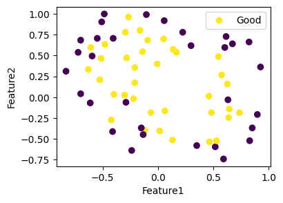
Visualize data

import matplotlib.pyplot as plt

fig, ax = plt.subplots(figsize=(4, 3))
ax.scatter(
    x=train_df["Feature1"], y=train_df["Feature2"], c=train_df["Label"], label="Good"
)
ax.set_xlabel("Feature1")
ax.set_ylabel("Feature2")
ax.legend()
plt.show()

Lift the 2D data

Logistic regression is an example of a binary classifier, where the output takes one of the two values 0 or 1 for each data point. We call the two values classes.

As we see from the plot, a linear separation of the classes is not reasonable. We lift the 2D data into $\mathbf{R}^{28}$ via sums of monomials of degrees up to 6.

def safe_pow(x, p):
    if np.min(x) > 0 or p.is_integer():
        return x**p
    x1 = np.array(x)
    x2 = np.array(x)
    x1[x1 < 0] = -((-x1[x1 < 0]) ** p)
    x2[x2 > 0] = x2[x2 > 0] ** p
    x2[x < 0] = x1[x < 0]
    return x2


def lift_to_degree(x, y, deg, step=1):
    result = pd.DataFrame()
    for i in np.arange(0, deg + step, step):
        for j in np.arange(0, i + step, step):
            temp = safe_pow(x, i) + safe_pow(y, (i - j))
            result[f"V{i}{i-j}"] = temp
    return result

degree_lift = 6
degree_step = 1
train_df_lifted = lift_to_degree(
    train_df["Feature1"], train_df["Feature2"], degree_lift, degree_step
)
test_df_lifted = lift_to_degree(
    test_df["Feature1"], test_df["Feature2"], degree_lift, degree_step
)
display(train_df_lifted)

	V00	V11	V10	V22	V21	V20	V33	V32	V31	V30	...	V52	V51	V50	V66	V65	V64	V63	V62	V61	V60
4	2.0	-0.047610	0.48675	0.480246	0.729066	1.263426	-0.034243	0.081617	0.330437	0.864797	...	0.181205	0.430024	0.964384	0.028473	0.040170	0.065291	0.119240	0.235101	0.483920	1.018280
90	2.0	0.396750	0.49251	1.075196	1.161786	1.257546	0.608650	0.686948	0.773538	0.869298	...	0.783988	0.870578	0.966338	0.563724	0.621614	0.685635	0.756435	0.834733	0.921323	1.017083
56	2.0	-0.236283	0.78053	0.048450	0.031354	1.048167	-0.010576	-0.010289	-0.027384	0.989429	...	-0.000227	-0.017322	0.999491	0.000112	0.000112	0.000112	0.000107	0.000394	-0.016701	1.000112
85	2.0	-0.655913	0.30242	0.488354	0.528285	1.486618	-0.339383	-0.337719	-0.297788	0.660545	...	-0.163449	-0.123518	0.834815	0.115230	0.115230	0.115233	0.115302	0.116966	0.156897	1.115230
28	2.0	0.407230	0.86118	0.317442	0.565321	1.019271	0.160141	0.295495	0.543375	0.997325	...	0.298119	0.545998	0.999948	0.026516	0.048554	0.088913	0.162823	0.298178	0.546057	1.000007
...	...	...	...	...	...	...	...	...	...	...	...	...	...	...	...	...	...	...	...	...	...
6	2.0	-0.363683	0.60196	0.159616	0.192793	1.158436	-0.063023	-0.061883	-0.028707	0.936936	...	-0.008811	0.024365	0.990008	0.003977	0.003977	0.003978	0.004018	0.005157	0.038334	1.003977
16	2.0	0.705210	1.16647	0.317953	0.566452	1.027712	0.160978	0.294854	0.543353	1.004613	...	0.290369	0.538868	1.000128	0.024471	0.045405	0.084261	0.156386	0.290262	0.538761	1.000021
26	2.0	-0.069810	1.46601	0.504268	-0.318655	1.217165	-0.052634	0.388304	-0.434619	1.101201	...	0.309080	-0.513843	1.021977	0.033907	-0.033925	0.092670	-0.143594	0.297345	-0.525578	1.010242
81	2.0	-0.581160	0.86694	0.218499	-0.430395	1.017705	-0.092331	0.198438	-0.450456	0.997644	...	0.200752	-0.448142	0.999958	0.008101	-0.018061	0.040324	-0.089970	0.200799	-0.448094	1.000006
30	2.0	0.697170	0.73445	0.997347	1.033237	1.070517	0.873552	0.908104	0.943994	0.981274	...	0.925509	0.961400	0.998680	0.796510	0.827340	0.859364	0.892628	0.927180	0.963071	1.000351

67 rows × 28 columns

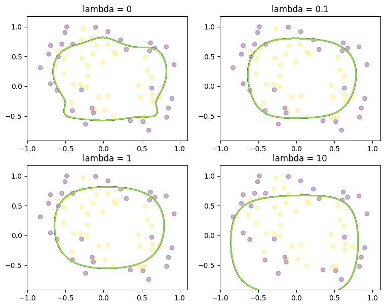
Solve and visualize

def plot_regression(dataset, lambd, theta, ax):
    x, y, c = dataset["Feature1"], dataset["Feature2"], dataset["Label"]
    ax.scatter(x, y, c=c, label="Good", alpha=0.3)
    x0, y0, x1, y1 = min(x), min(y), max(x), max(y)
    xd = (x1 - x0) / 10
    yd = (y1 - y0) / 10
    xr = np.linspace(x0 - xd, x1 + xd, 500)
    yr = np.linspace(y0 - xd, y1 + xd, 500)
    X, Y = np.meshgrid(xr, yr)  # grid of points
    X1 = np.reshape(X, (500 * 500))
    Y1 = np.reshape(Y, (500 * 500))
    X1Y1lft = lift_to_degree(X1, Y1, degree_lift, degree_step)
    theta_by_X1Y1 = theta.T @ X1Y1lft.T
    Z = (theta_by_X1Y1.values > 0).astype(int).reshape(500, 500)
    ax.contour(X, Y, Z)
    ax.set_title(f"lambda = {lambd}")

def solve_and_subplot(train_df, train_df_lifted, lambd, ax, mdl, slv):
    theta, tm = logistic_regression(train_df["Label"], train_df_lifted, lambd, mdl, slv)
    print(f"Solving time: {tm:.2f} sec.")
    plot_regression(train_df, lambd, theta, ax)
    return theta, tm

def benchmark_lambda(train_df, train_df_lifted, modfile, solver):
    fig, ax = plt.subplots(2, 2, figsize=(9, 7))
    theta = {}
    theta[0], _ = solve_and_subplot(
        train_df, train_df_lifted, 0, ax[0, 0], modfile, solver
    )
    theta[0.1], _ = solve_and_subplot(
        train_df, train_df_lifted, 0.1, ax[0, 1], modfile, solver
    )
    theta[1], _ = solve_and_subplot(
        train_df, train_df_lifted, 1, ax[1, 0], modfile, solver
    )
    theta[10], _ = solve_and_subplot(
        train_df, train_df_lifted, 10, ax[1, 1], modfile, solver
    )
    plt.show()
    return theta

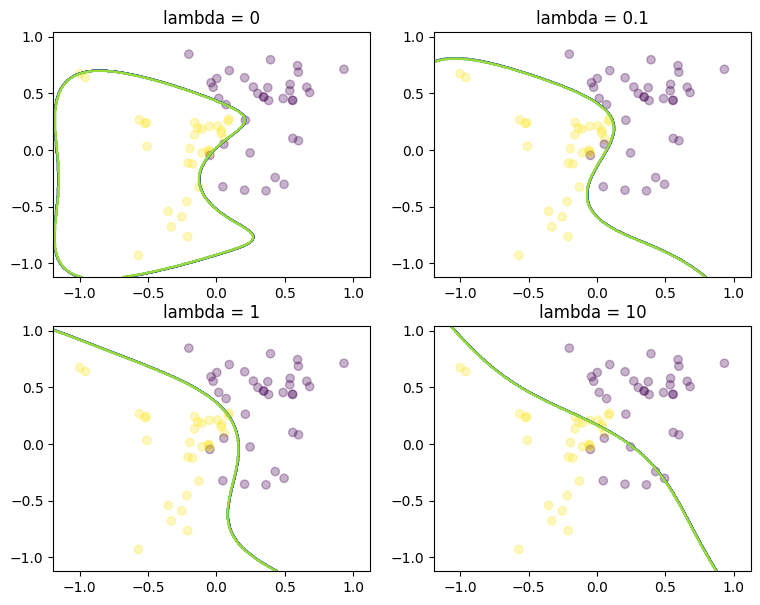
theta_logistic_ipopt = benchmark_lambda(
    train_df, train_df_lifted, "logistic_regression.mod", "ipopt"
)

Ipopt 3.12.13: Optimal Solution Found
Solving time: 0.05 sec.
Ipopt 3.12.13: Optimal Solution Found
Solving time: 0.05 sec.
Ipopt 3.12.13: Optimal Solution Found
Solving time: 0.04 sec.
Ipopt 3.12.13: Optimal Solution Found
Solving time: 0.11 sec.

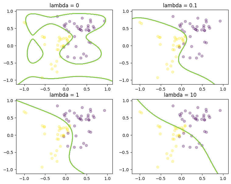
theta_conic_ipopt = benchmark_lambda(
    train_df, train_df_lifted, "logistic_regression_conic.mod", "ipopt"
)

Ipopt 3.12.13: Optimal Solution Found
Solving time: 0.37 sec.
Ipopt 3.12.13: Optimal Solution Found
Solving time: 0.24 sec.
Ipopt 3.12.13: Optimal Solution Found
Solving time: 0.20 sec.
Ipopt 3.12.13: Optimal Solution Found
Solving time: 0.28 sec.

theta_conic_mosek = benchmark_lambda(
    train_df, train_df_lifted, "logistic_regression_conic.mod", "mosek"
)

MOSEK 10.0.43: optimal; objective 28.81852891
0 simplex iterations
12 barrier iterations
Solving time: 0.04 sec.
MOSEK 10.0.43: optimal; objective 30.90498809
0 simplex iterations
9 barrier iterations
Solving time: 0.04 sec.
MOSEK 10.0.43: optimal; objective 35.10091469
0 simplex iterations
10 barrier iterations
Solving time: 0.05 sec.
MOSEK 10.0.43: optimal; objective 46.19055461
0 simplex iterations
12 barrier iterations
Solving time: 0.04 sec.

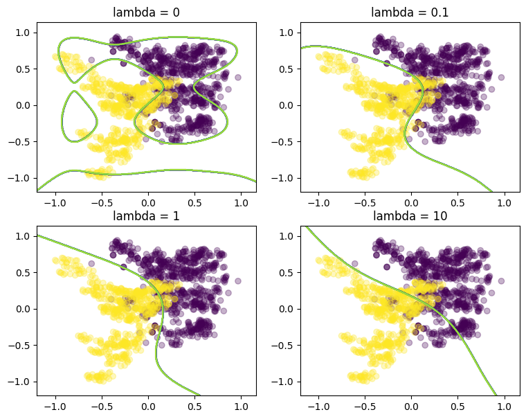
Evaluate perfornace the optimal $\theta$ for each lambda on the test set

theta = theta_conic_mosek  # using theta from the conic model with MOSEK
fig, axes = plt.subplots(2, 2, figsize=(9, 7))
for lambd, axis in zip([0, 0.1, 1, 10], np.ravel(axes).tolist()):
    plot_regression(test_df, lambd, theta[lambd], axis)
plt.show()

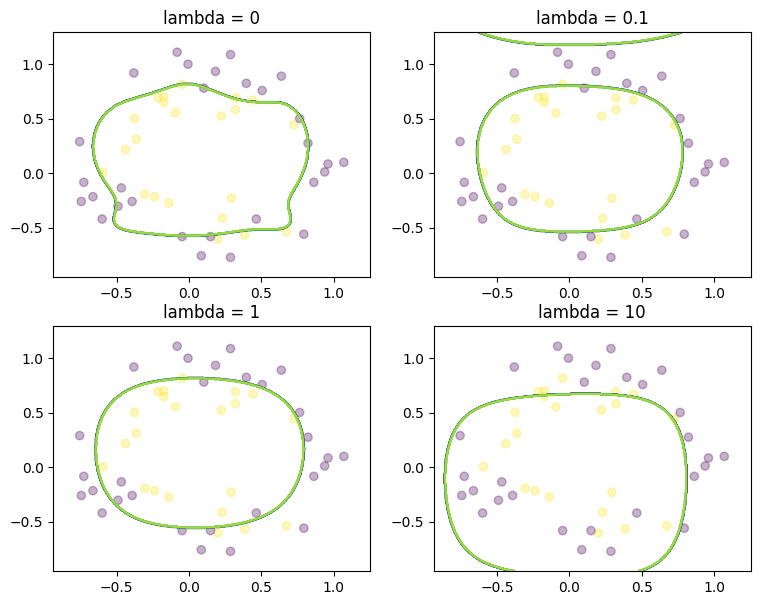
# Check the accuracy for each lambda
for lambd in sorted(theta):
    result_df = test_df.copy()
    result_df["pred"] = test_df_lifted.dot(theta[lambd]) >= 0
    accuracy = sum(result_df["Label"] == result_df["pred"]) / len(result_df)
    print(f"accuracy with lambda={lambd:5.2f}: {accuracy*100:.2f}%")

accuracy with lambda= 0.00: 74.51%
accuracy with lambda= 0.10: 82.35%
accuracy with lambda= 1.00: 82.35%
accuracy with lambda=10.00: 62.75%

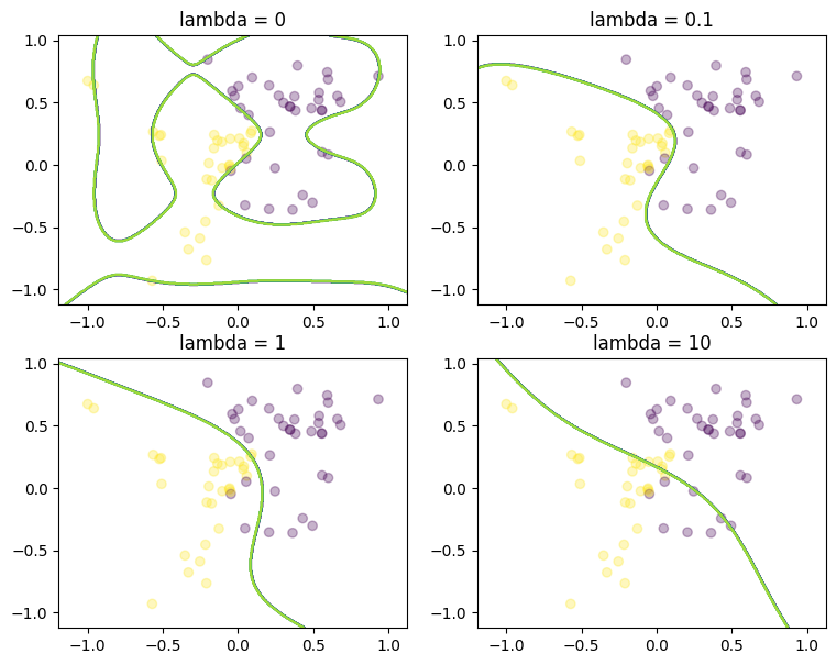
2. A larger data set

We consider a larger data set from [2], explored in Chapter 6 of the book Mathematical Optimization with AMPL in Python. The following data set contains data from a collection of known genuine and known counterfeit banknote specimens. The data includes four continuous statistical measures obtained from the wavelet transform of banknote images named “variance”, “skewness”, “curtosis”, and “entropy”, and a binary variable named “class” which is 0 if genuine and 1 if counterfeit.

# read data set
df = pd.read_csv(
    "https://raw.githubusercontent.com/ampl/colab.ampl.com/master/datasets/regression/data_banknote_authentication.csv",
    names=["variance", "skewness", "curtosis", "entropy", "class"],
    header=None,
)
df.name = "Banknotes"
display(df.T)  # Transposed

	0	1	2	3	4	5	6	7	8	9	...	1362	1363	1364	1365	1366	1367	1368	1369	1370	1371
variance	3.62160	4.5459	3.86600	3.4566	0.32924	4.3684	3.59120	2.09220	3.20320	1.53560	...	-2.166800	-1.16670	-2.83910	-4.50460	-2.41000	0.40614	-1.38870	-3.7503	-3.5637	-2.54190
skewness	8.66610	8.1674	-2.63830	9.5228	-4.45520	9.6718	3.01290	-6.81000	5.75880	9.17720	...	1.593300	-1.42370	-6.63000	-5.81260	3.74330	1.34920	-4.87730	-13.4586	-8.3827	-0.65804
curtosis	-2.80730	-2.4586	1.92420	-4.0112	4.57180	-3.9606	0.72888	8.46360	-0.75345	-2.27180	...	0.045122	2.92410	10.48490	10.88670	-0.40215	-1.45010	6.47740	17.5932	12.3930	2.68420
entropy	-0.44699	-1.4621	0.10645	-3.5944	-0.98880	-3.1625	0.56421	-0.60216	-0.61251	-0.73535	...	-1.678000	0.66119	-0.42113	-0.52846	-1.29530	-0.55949	0.34179	-2.7771	-1.2823	1.19520
class	0.00000	0.0000	0.00000	0.0000	0.00000	0.0000	0.00000	0.00000	0.00000	0.00000	...	1.000000	1.00000	1.00000	1.00000	1.00000	1.00000	1.00000	1.0000	1.0000	1.00000

5 rows × 1372 columns

Select features

From the 4 features we select 2 to be able to visualize the results. Similar to the small example, we lift the 2D data into $\mathbf{R}^{28}$ via sums of monomials of degrees up to 6.

# select training features
features_df = df[["variance", "skewness", "class"]].copy()
features_df.columns = ["Feature1", "Feature2", "Label"]

# normalize
features_df["Feature1"] /= features_df["Feature1"].abs().max()
features_df["Feature2"] /= features_df["Feature2"].abs().max()

# slit train/test sets
train_df, test_df = split_df(features_df, demo_limits=True)

# lift the 2D data
degree_lift = 6
degree_step = 1
train_df_lifted = lift_to_degree(
    train_df["Feature1"], train_df["Feature2"], degree_lift, degree_step
)
test_df_lifted = lift_to_degree(
    test_df["Feature1"], test_df["Feature2"], degree_lift, degree_step
)
# display(train_df_lifted)

Solve

theta_logistic_ipopt = benchmark_lambda(
    train_df, train_df_lifted, "logistic_regression.mod", "ipopt"
)

Ipopt 3.12.13: Optimal Solution Found
Solving time: 0.06 sec.
Ipopt 3.12.13: Optimal Solution Found
Solving time: 0.04 sec.
Ipopt 3.12.13: Optimal Solution Found
Solving time: 0.04 sec.
Ipopt 3.12.13: Optimal Solution Found
Solving time: 0.03 sec.

theta_conic_ipopt = benchmark_lambda(
    train_df, train_df_lifted, "logistic_regression_conic.mod", "ipopt"
)

Ipopt 3.12.13: Optimal Solution Found
Solving time: 0.77 sec.
Ipopt 3.12.13: Optimal Solution Found
Solving time: 0.30 sec.
Ipopt 3.12.13: Optimal Solution Found
Solving time: 0.24 sec.
Ipopt 3.12.13: Optimal Solution Found
Solving time: 0.32 sec.

theta_conic_mosek = benchmark_lambda(
    train_df, train_df_lifted, "logistic_regression_conic.mod", "mosek"
)

MOSEK 10.0.43: optimal, stalling; objective 5.47048488e-06
0 simplex iterations
44 barrier iterations
Solving time: 0.08 sec.
MOSEK 10.0.43: optimal; objective 9.118865748
0 simplex iterations
22 barrier iterations
Solving time: 0.05 sec.
MOSEK 10.0.43: optimal; objective 18.77638933
0 simplex iterations
12 barrier iterations
Solving time: 0.04 sec.
MOSEK 10.0.43: optimal; objective 39.26932934
0 simplex iterations
13 barrier iterations
Solving time: 0.05 sec.

Evaluate perfornace the optimal $\theta$ for each lambda on the test set

theta = theta_conic_mosek  # using theta from the conic model with MOSEK
fig, axes = plt.subplots(2, 2, figsize=(9, 7))
for lambd, axis in zip([0, 0.1, 1, 10], np.ravel(axes).tolist()):
    plot_regression(test_df, lambd, theta[lambd], axis)
plt.show()

# Check the accuracy for each lambda
for lambd in sorted(theta):
    result_df = test_df.copy()
    result_df["pred"] = test_df_lifted.dot(theta[lambd]) >= 0
    accuracy = sum(result_df["Label"] == result_df["pred"]) / len(result_df)
    print(f"accuracy with lambda={lambd:5.2f}: {accuracy*100:.2f}%")

accuracy with lambda= 0.00: 81.46%
accuracy with lambda= 0.10: 92.34%
accuracy with lambda= 1.00: 91.42%
accuracy with lambda=10.00: 85.44%

Discussion

Logistic regression can be modeled as a convex nonlinear optimization problem.

We considered two examples with none, medium and strong regularization (small, medium, large lambda). Without regularization we get obvious overfitting and numerical issues in the solvers.

previous

Largest small polygon

next

Magic sequences