Network design with redundancy

Description: Design of an electricity transportation network provides enough redundancy, so that a break of one component does not prevent any user from receiving electricity. The approach also works for similar distribution networks and can potentially be used in the design of military logistic networks.

Tags: electric-grid, military

Notebook author: Filipe Brandão <fdabrandao@gmail.com>

Model author: Filipe Brandão

# Install dependencies
%pip install -q amplpy matplotlib networkx

# Google Colab & Kaggle integration
from amplpy import AMPL, ampl_notebook

ampl = ampl_notebook(
    modules=["gurobi", "highs"],  # modules to install
    license_uuid="default",  # license to use
)  # instantiate AMPL object and register magics

Network

# Data typically would come from some source such as csv/excel files, databases, etc.
# In this example the data is in the python dictionaries below
coordinates = {
    1: (300, 100),
    2: (600, 100),
    3: (700, 200),
    4: (900, 700),
    5: (500, 500),
    6: (400, 900),
    7: (150, 100),
    8: (400, 80),
    9: (950, 70),
    10: (30, 120),
    11: (600, 300),
    12: (20, 450),
    13: (300, 500),
    14: (950, 450),
    15: (70, 800),
    16: (350, 750),
    17: (500, 750),
    18: (600, 800),
    19: (600, 900),
    20: (750, 750),
    21: (850, 950),
}
demsup = {
    1: -900,
    2: -500,
    3: -1200,
    4: -450,
    5: -750,
    6: -1200,
    7: 200,
    8: 300,
    9: 200,
    10: 250,
    11: 300,
    12: 250,
    13: 300,
    14: 300,
    15: 250,
    16: 150,
    17: 250,
    18: 300,
    19: 100,
    20: 250,
    21: 250,
}
capacity = 1000

import matplotlib.pyplot as plt


def dist(u, v):
    (x1, y1), (x2, y2) = coordinates[u], coordinates[v]
    return ((x2 - x1) ** 2 + (y2 - y1) ** 2) ** 0.5


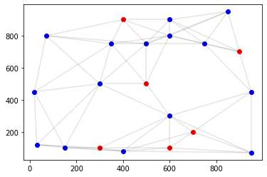
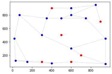
def draw_network(edges, coordinates, balance):
    xl, yl = zip(*[coordinates[u] for u in [u for u in balance if balance[u] < 0]])
    plt.scatter(xl, yl, color="red")
    xl, yl = zip(*[coordinates[u] for u in [u for u in balance if balance[u] >= 0]])
    plt.scatter(xl, yl, color="blue")
    for u, v in edges:
        (x1, y1), (x2, y2) = coordinates[int(u)], coordinates[int(v)]
        plt.plot([x1, x2], [y1, y2], "k-", alpha=0.1)

N = list(coordinates.keys())
L = set()
for u in N:
    # from each note, we only consider edges to the closest 5 other nodes
    lst = sorted([(dist(u, v), v) for v in N if v != u])[:5]
    for _, v in lst:
        L.add((min(u, v), max(u, v)))
L = list(L)
draw_network(L, coordinates, demsup)
cost = {(u, v): dist(u, v) for (u, v) in L}

Model for single-node failure

We consider a simplified network (i.e., we ignore the existence of transformers near the cities among other components). Let $E$ be the set of edges (i.e., undirected), and $A$ be the set of (directed) arcs connecting each pair $i,j$. The parameters of this model are the arc capacities $U_{ij}=1000$ (Megawatts), nodes production or consumption $b_i$ (negative value means that there is energy production in the node), and the cost of each line $c_{ij}$, equal to one million euro per kilometer of the edge $(i,j)$.

We define the following variables:

• $y_{ij}$ is 1 if edge ${i,j}$ is constructed, 0 otherwise;

• $f_{ij}$ is the flow on arc $(i,j)$ if there is no failure on any other arc;

• $f_{ij}^{u}$ is the flow on edge ${i,j}$ if there is a failure on node $u$;

The objective is to minimize total cost of connecting the nodes: $$\textrm{minimize } \sum_{{i,j} \in E} c_{ij} y_{ij}$$

The restrictions are the following:

• There can only be flow if the edge was built: $$f_{ij} \leq U_{ij} y_{ij}, ;;; \forall {i,j} \in E$$ $$f_{ji} \leq U_{ji} y_{ij}, ;;; \forall {i,j} \in E$$

• Demand and production capacity satisfaction: $$\sum_{(i,j) \in A} f_{ij} - \sum_{(j,i) \in A} f_{ji} \geq b_i, ;;; \forall i \in N$$

• There cannot be flow through node $u$ when it fails: $$\sum_{(i,u) \in A} f_{iu}^u + \sum_{(u,j) \in A} f_{uj}^u = 0, ;;; \forall u \in N$$

• If node $u$ fails, flow through remaining edges and satisfy demand: $$\sum_{(i,j) \in A} f_{ij}^u - \sum_{(j,i) \in A} f_{ji}^u \geq b_i, ;;; \forall u \in N, \forall i \in N \setminus {u}$$

• Arcs needed when node $u$ fails must be built: $$f_{ij}^u \leq U_{ij} y_{ij}, ;;; \forall {i,j} \in E$$ $$f_{ji}^u \leq U_{ji} y_{ij}, ;;; \forall {i,j} \in E$$

%%ampl_eval
set N;                                     # nodes
set L within N cross N;                    # set of links
set A = L union setof {(i,j) in L} (j,i);  # arcs (directed)

param demsup{N};   # demand (positive) or supply (negative)
param cost{L};     # cost to build a link
param capacity;    # capacity of links

var Build {L} binary;   # Build[i,j] = 1 iff link btw i & j is built
var Flow {A} >= 0;      # Flow[i,j] is flow from i to j

minimize TotalBuildCost:
    sum {(i,j) in L} cost[i,j] * Build[i,j];

subject to Balance {i in N}:
    sum {(j,i) in A} Flow[j,i] - sum{(i,j) in A} Flow[i,j] >= demsup[i];

subject to ArcExists1 {(i,j) in L}:
    Flow[i,j] <= Build[i,j] * capacity;
subject to ArcExists2 {(i,j) in L}:
    Flow[j,i] <= Build[i,j] * capacity;

var FlRm {A,N} >= 0; # FlRm[i,j,rn] is flow from i to j when node rn is removed

subject to RemoveNode {rm in N}:
    sum {(i,rm) in A} FlRm[i,rm,rm] + sum {(rm,j) in A} FlRm[rm,j,rm] = 0;

subject to BalanceRm {i in N, rm in N: i != rm}:
    sum {(j,i) in A} FlRm[j,i,rm] - sum {(i,j) in A} FlRm[i,j,rm] >= demsup[i];

subject to ArcExistsRm1 {(i,j) in L, rm in N}:
    FlRm[i,j,rm] <= Build[i,j] * capacity;
subject to ArcExistsRm2 {(i,j) in L, rm in N}:
    FlRm[j,i,rm] <= Build[i,j] * capacity;

Load data

ampl.set["N"] = N
ampl.set["L"] = L
ampl.param["capacity"] = capacity
ampl.param["cost"] = cost
ampl.param["demsup"] = demsup

ampl.param["demsup"].to_pandas()

	demsup
1.0	-900.0
2.0	-500.0
3.0	-1200.0
4.0	-450.0
5.0	-750.0
6.0	-1200.0
7.0	200.0
8.0	300.0
9.0	200.0
10.0	250.0
11.0	300.0
12.0	250.0
13.0	300.0
14.0	300.0
15.0	250.0
16.0	150.0
17.0	250.0
18.0	300.0
19.0	100.0
20.0	250.0
21.0	250.0

Solve

ampl.option["solver"] = "gurobi"
ampl.option["gurobi_options"] = "outlev=1 timelim=10"
ampl.option["highs_options"] = "outlev=1 timelim=60"
ampl.solve()

Gurobi 10.0.0: Set parameter OutputFlag to value 1
tech:outlev=1
Set parameter TimeLimit to value 10
lim:time=10
Set parameter InfUnbdInfo to value 1
Gurobi Optimizer version 10.0.0 build v10.0.0rc2 (linux64)

CPU model: Intel(R) Xeon(R) CPU @ 2.20GHz, instruction set [SSE2|AVX|AVX2]
Thread count: 1 physical cores, 2 logical processors, using up to 2 threads

Optimize a model with 2921 rows, 2542 columns and 9920 nonzeros
Model fingerprint: 0x250da436
Variable types: 2480 continuous, 62 integer (0 binary)
Coefficient statistics:
  Matrix range     [1e+00, 1e+03]
  Objective range  [1e+02, 6e+02]
  Bounds range     [1e+00, 1e+00]
  RHS range        [1e+02, 1e+03]

User MIP start did not produce a new incumbent solution
User MIP start violates constraint R2486 by 200.000000000

Found heuristic solution: objective 16794.262944
Presolve time: 0.01s
Presolved: 2921 rows, 2542 columns, 9920 nonzeros
Variable types: 2480 continuous, 62 integer (62 binary)

Root relaxation: objective 1.807099e+03, 2628 iterations, 0.07 seconds (0.04 work units)
Another try with MIP start

    Nodes    |    Current Node    |     Objective Bounds      |     Work
 Expl Unexpl |  Obj  Depth IntInf | Incumbent    BestBd   Gap | It/Node Time

     0     0 1807.09948    0   43 16794.2629 1807.09948  89.2%     -    0s
H    0     0                    11702.196790 1807.09948  84.6%     -    0s
     0     0 2469.18592    0   47 11702.1968 2469.18592  78.9%     -    0s
     0     0 2643.27037    0   44 11702.1968 2643.27037  77.4%     -    0s
     0     0 2704.46316    0   46 11702.1968 2704.46316  76.9%     -    0s
     0     0 2711.22061    0   48 11702.1968 2711.22061  76.8%     -    0s
     0     0 2711.31011    0   47 11702.1968 2711.31011  76.8%     -    0s
     0     0 3053.78715    0   52 11702.1968 3053.78715  73.9%     -    0s
     0     0 3150.77649    0   47 11702.1968 3150.77649  73.1%     -    0s
     0     0 3189.94134    0   47 11702.1968 3189.94134  72.7%     -    0s
     0     0 3216.07767    0   48 11702.1968 3216.07767  72.5%     -    0s
     0     0 3224.13982    0   45 11702.1968 3224.13982  72.4%     -    0s
     0     0 3227.13460    0   49 11702.1968 3227.13460  72.4%     -    0s
     0     0 3228.74714    0   51 11702.1968 3228.74714  72.4%     -    0s
     0     0 3228.74714    0   51 11702.1968 3228.74714  72.4%     -    0s
     0     0 3385.52331    0   48 11702.1968 3385.52331  71.1%     -    1s
     0     0 3449.37050    0   48 11702.1968 3449.37050  70.5%     -    1s
     0     0 3455.04358    0   45 11702.1968 3455.04358  70.5%     -    1s
     0     0 3463.22356    0   45 11702.1968 3463.22356  70.4%     -    1s
     0     0 3472.54233    0   46 11702.1968 3472.54233  70.3%     -    1s
     0     0 3472.74387    0   45 11702.1968 3472.74387  70.3%     -    1s
     0     0 3539.64192    0   47 11702.1968 3539.64192  69.8%     -    1s
     0     0 3583.42134    0   46 11702.1968 3583.42134  69.4%     -    1s
     0     0 3653.13982    0   45 11702.1968 3653.13982  68.8%     -    1s
     0     0 3675.06156    0   45 11702.1968 3675.06156  68.6%     -    1s
     0     0 3675.95141    0   49 11702.1968 3675.95141  68.6%     -    1s
     0     0 3741.33194    0   43 11702.1968 3741.33194  68.0%     -    1s
H    0     0                    11592.835343 3741.33194  67.7%     -    1s
     0     0 3746.91573    0   47 11592.8353 3746.91573  67.7%     -    1s
     0     0 3749.36524    0   48 11592.8353 3749.36524  67.7%     -    1s
     0     0 3749.65024    0   48 11592.8353 3749.65024  67.7%     -    1s
     0     0 3787.58978    0   42 11592.8353 3787.58978  67.3%     -    2s
     0     0 3793.15188    0   46 11592.8353 3793.15188  67.3%     -    2s
     0     0 3794.69683    0   45 11592.8353 3794.69683  67.3%     -    2s
     0     0 3803.28176    0   44 11592.8353 3803.28176  67.2%     -    2s
     0     0 3804.35041    0   45 11592.8353 3804.35041  67.2%     -    2s
     0     0 3829.65282    0   40 11592.8353 3829.65282  67.0%     -    2s
H    0     0                    10693.991491 3829.65282  64.2%     -    2s
     0     0 3831.17570    0   42 10693.9915 3831.17570  64.2%     -    2s
     0     0 3831.35668    0   42 10693.9915 3831.35668  64.2%     -    2s
     0     0 3834.79460    0   40 10693.9915 3834.79460  64.1%     -    2s
     0     0 3834.79460    0   40 10693.9915 3834.79460  64.1%     -    2s
H    0     0                    9356.1657294 3834.79460  59.0%     -    2s
     0     2 3835.00936    0   40 9356.16573 3835.00936  59.0%     -    2s
H    7     7                    8985.3134720 3843.39902  57.2%   370    2s
H    8     8                    8694.8625152 3843.39902  55.8%   362    2s
H   11    11                    8623.1986429 3843.39902  55.4%   429    2s
H   14    14                    8103.5678236 3843.39902  52.6%   420    3s
H   15    15                    7722.7791683 3843.39902  50.2%   400    3s
H   19    19                    7578.1948749 3843.39902  49.3%   361    3s
H   20    20                    7546.1975208 3843.39902  49.1%   352    3s
H   21    21                    6801.2959752 3843.39902  43.5%   342    3s
H   22    22                    6355.3139128 3843.39902  39.5%   333    3s
H   24    24                    5920.8068276 3843.39902  35.1%   316    3s
H   33    33                    5728.8456732 3843.39902  32.9%   273    3s
H   37    37                    5417.5756422 3843.39902  29.1%   249    3s
H   38    38                    5136.4360751 3843.39902  25.2%   243    3s
H   40    40                    4844.8884803 3843.39902  20.7%   235    3s
*   45    41              36    4733.0850814 3843.39902  18.8%   212    3s
*  131   103              31    4669.4968467 3904.54048  16.4%   260    4s
   223   177     cutoff   22      4669.49685 3921.54998  16.0%   263    5s

Cutting planes:
  Gomory: 2
  MIR: 462
  Flow cover: 445
  Zero half: 12
  Relax-and-lift: 3

Explored 540 nodes (183571 simplex iterations) in 10.01 seconds (6.45 work units)
Thread count was 2 (of 2 available processors)

Solution count 10: 4669.5 4733.09 4844.89 ... 7546.2

Time limit reached
Best objective 4.669496846723e+03, best bound 3.963581515275e+03, gap 15.1176%
Gurobi 10.0.0: time limit, feasible solution
183571 simplex iterations
540 branching nodes
absmipgap=705.915, relmipgap=0.151176

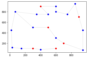
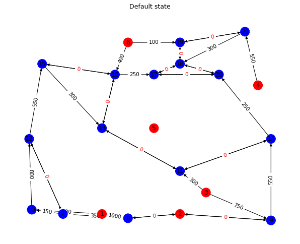
Display solution

d = ampl.get_data("{(i,j) in L: Build[i,j] > 0} Build[i,j]").to_dict()
draw_network(d.keys(), coordinates, demsup)

Display flows

import networkx as nx
import matplotlib.pyplot as plt


def draw_solution(flow, title):
    solution = {}
    edges = set(((min(u, v)), max(u, v)) for u, v in flow)
    for u, v in edges:
        f = flow.get((u, v), 0) - flow.get((v, u), 0)
        u, v = int(u), int(v)
        if abs(f) == 0:
            solution[(u, v)] = solution[(v, u)] = 0
        else:
            solution[(u, v) if f > 0 else (v, u)] = abs(f)
    G = nx.DiGraph()
    color_map = []
    for u in coordinates:
        G.add_node(u, pos=coordinates[u])
        color_map.append("red" if demsup[u] < 0 else "blue")
    G.add_edges_from(solution.keys())
    pos = nx.get_node_attributes(G, "pos")
    f = plt.figure(figsize=(10, 8), dpi=75)
    ax = f.add_subplot()
    ax.set_title(title)
    nx.draw(G, pos, with_labels=True, ax=ax, node_color=color_map)
    labels = nx.draw_networkx_edge_labels(
        G,
        pos,
        edge_labels={(u, v): f"{f:.0f}" for (u, v), f in solution.items() if f > 0},
    )
    labels = nx.draw_networkx_edge_labels(
        G,
        pos,
        edge_labels={(u, v): "0" for (u, v), f in solution.items() if f <= 0},
        font_color="red",
    )

draw_solution(
    ampl.get_data("{(i,j) in A: Build[min(i,j),max(i,j)] > 0} Flow[i,j]").to_dict(),
    "Default state",
)

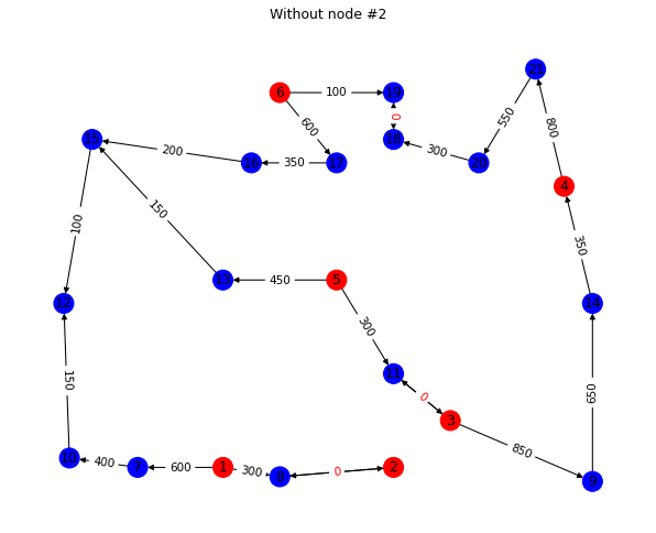
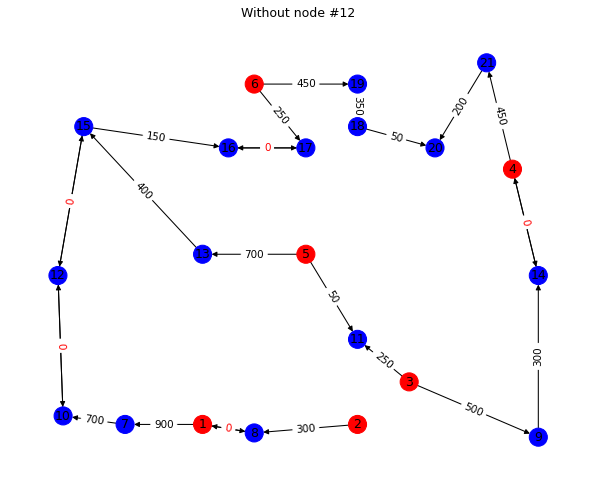
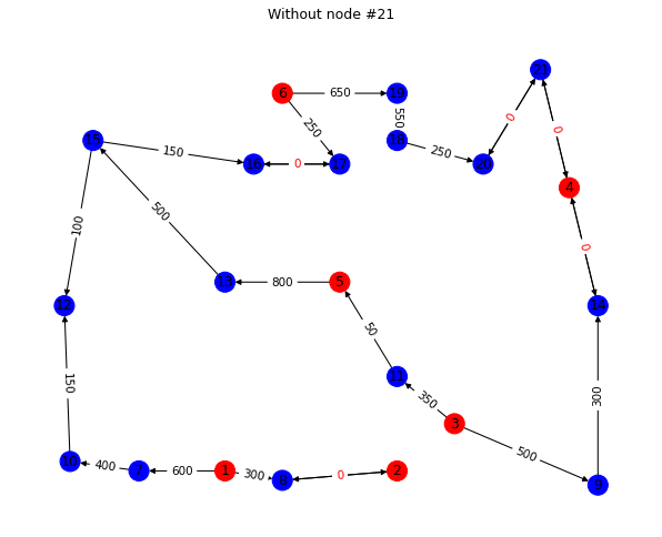
During failures

for u in N:
    draw_solution(
        ampl.get_data(
            "{(i,j) in A: Build[min(i,j),max(i,j)] > 0}" + f"FlRm[i,j,{u}]"
        ).to_dict(),
        title=f"Without node #{u}",
    )

<ipython-input-210-9a40522e9a71>:21: RuntimeWarning: More than 20 figures have been opened. Figures created through the pyplot interface (`matplotlib.pyplot.figure`) are retained until explicitly closed and may consume too much memory. (To control this warning, see the rcParam `figure.max_open_warning`).
  f = plt.figure(figsize=(10, 8), dpi=75)

Model for double-node failure

We define the following variables:

• $y_{ij}$ is 1 if edge ${i,j}$ is constructed, 0 otherwise;

• $f_{ij}$ is the flow on arc $(i,j)$ if there is no failure on any other arc;

• $f_{ij}^{uv}$ is the flow on edge ${i,j}$ if both nodes $u$ and $v$ fail;

The objective is to minimize total cost of connecting the nodes: $$\textrm{minimize } \sum_{{i,j} \in E} c_{ij} y_{ij}$$

The restrictions are the following:

• There can only be flow if the edge was built: $$f_{ij} \leq U_{ij} y_{ij}, ;;; \forall {i,j} \in E$$ $$f_{ji} \leq U_{ji} y_{ij}, ;;; \forall {i,j} \in E$$

• Demand and production capacity satisfaction: $$\sum_{(i,j) \in A} f_{ij} - \sum_{(j,i) \in A} f_{ji} \geq b_i, ;;; \forall i \in N$$

• There cannot be flow through nodes $u$ and $v$ when they fail: $$\sum_{(i,u) \in A} f_{iu}^{uv} + \sum_{(u,j) \in A} f_{uj}^{uv} + \sum_{(i,v) \in A} f_{iv}^{uv} + \sum_{(v,j) \in A} f_{vj}^{uv} = 0, ;;; \forall (u,v) \in N \times N$$

• If nodes $u$ and $v$ fail, flow through remaining edges and satisfy demand: $$\sum_{(i,j) \in A} f_{ij}^{uv} - \sum_{(j,i) \in A} f_{ji}^{uv} \geq b_i, ;;; \forall (u,v) \in N \times N, \forall i \in N \setminus {u,v}$$

• Arcs needed when node $u$ fails must be built: $$f_{ij}^{uv} \leq U_{ij} y_{ij}, ;;; \forall (u,v) \in N \times N, \forall {i,j} \in E$$ $$f_{ji}^{uv} \leq U_{ji} y_{ij}, ;;; \forall (u,v) \in N \times N, \forall {i,j} \in E$$

%%ampl_eval
reset;
set N;                                     # nodes
set L within N cross N;                    # set of links
set A = L union setof {(i,j) in L} (j,i);  # arcs (directed)

param demsup{N};   # demand (positive) or supply (negative)
param cost{L};     # cost to build a link
param capacity;    # capacity of links

var Build {L} binary;   # Build[i,j] = 1 iff link btw i & j is built
var Flow {A} >= 0;      # Flow[i,j] is flow from i to j

minimize TotalBuildCost:
    sum {(i,j) in L} cost[i,j] * Build[i,j];

subject to Balance {i in N}:
    sum {(j,i) in A} Flow[j,i] - sum{(i,j) in A} Flow[i,j] >= demsup[i];

subject to ArcExists1 {(i,j) in L}:
    Flow[i,j] <= Build[i,j] * capacity;
subject to ArcExists2 {(i,j) in L}:
    Flow[j,i] <= Build[i,j] * capacity;

set RNs := {rn1 in N, rn2 in N : rn1 < rn2}; # pairs or nodes that may fail

var frns{A, RNs} >= 0;
s.t. RemoveNodes{(rn1,rn2) in RNs}:
    sum{(i1,rn1) in A} frns[i1,rn1,rn1,rn2] + sum{(rn1,j1) in A} frns[rn1,j1,rn1,rn2]
    + sum{(i2,rn2) in A} frns[i2,rn2,rn1,rn2] + sum{(rn2,j2) in A} frns[rn2,j2,rn1,rn2] = 0;
s.t. BalanceRN{u in N, (rn1,rn2) in RNs: u != rn1 && u != rn2}:
    sum{(i,u) in A} frns[i,u,rn1,rn2] - sum{(u,j) in A} frns[u,j,rn1,rn2] >= demsup[u];
s.t. ArcExistsRN1{(i,j) in L, (rn1,rn2) in RNs}:
    frns[i,j,rn1,rn2] <= Build[i,j] * capacity;
s.t. ArcExistsRN2{(i,j) in L, (rn1,rn2) in RNs}:
    frns[j,i,rn1,rn2] <= Build[i,j] * capacity;

ampl.set["N"] = N
ampl.set["L"] = L
ampl.param["cost"] = cost
ampl.param["capacity"] = capacity
# The power production has to be higher in order to have feasible solutions if two power stations fail
demsup = {
    1: -1900,
    2: -1500,
    3: -2200,
    4: -1450,
    5: -1750,
    6: -2200,
    7: 200,
    8: 300,
    9: 200,
    10: 250,
    11: 300,
    12: 250,
    13: 300,
    14: 300,
    15: 250,
    16: 150,
    17: 250,
    18: 300,
    19: 100,
    20: 250,
    21: 250,
}
ampl.param["demsup"] = demsup

ampl.option["solver"] = "gurobi"
ampl.option["gurobi_options"] = "outlev=1 timelim=60"
ampl.option["highs_options"] = "outlev=1 timelim=60"
ampl.solve()

Gurobi 10.0.0: Set parameter OutputFlag to value 1
tech:outlev=1
Set parameter TimeLimit to value 60
lim:time=60
Set parameter InfUnbdInfo to value 1
Gurobi Optimizer version 10.0.0 build v10.0.0rc2 (linux64)

CPU model: Intel(R) Xeon(R) CPU @ 2.20GHz, instruction set [SSE2|AVX|AVX2]
Thread count: 1 physical cores, 2 logical processors, using up to 2 threads

Optimize a model with 25339 rows, 21390 columns and 85312 nonzeros
Model fingerprint: 0xd5811b0f
Variable types: 21328 continuous, 62 integer (0 binary)
Coefficient statistics:
  Matrix range     [1e+00, 1e+03]
  Objective range  [1e+02, 6e+02]
  Bounds range     [1e+00, 1e+00]
  RHS range        [1e+02, 2e+03]

User MIP start did not produce a new incumbent solution
User MIP start violates constraint R21334 by 200.000000000

Found heuristic solution: objective 16902.932489
Presolve removed 75 rows and 73 columns
Presolve time: 0.14s
Presolved: 25264 rows, 21317 columns, 85046 nonzeros
Variable types: 21255 continuous, 62 integer (62 binary)

Root relaxation: objective 2.517919e+03, 21610 iterations, 1.01 seconds (0.60 work units)
Another try with MIP start

    Nodes    |    Current Node    |     Objective Bounds      |     Work
 Expl Unexpl |  Obj  Depth IntInf | Incumbent    BestBd   Gap | It/Node Time

H    0     0                    8101.4200418 2517.91882  68.9%     -    1s
     0     0 2517.91882    0   54 8101.42004 2517.91882  68.9%     -    1s
     0     0 3448.93515    0   47 8101.42004 3448.93515  57.4%     -    2s
H    0     0                    7267.5117591 3448.93515  52.5%     -    3s
     0     0 3575.71285    0   46 7267.51176 3575.71285  50.8%     -    3s
     0     0 3637.56509    0   46 7267.51176 3637.56509  49.9%     -    4s
     0     0 3682.40497    0   50 7267.51176 3682.40497  49.3%     -    4s
     0     0 3683.64874    0   49 7267.51176 3683.64874  49.3%     -    4s
     0     0 3683.86016    0   49 7267.51176 3683.86016  49.3%     -    5s
     0     0 4158.64619    0   54 7267.51176 4158.64619  42.8%     -    6s
     0     0 4500.82024    0   48 7267.51176 4500.82024  38.1%     -    7s
     0     0 4513.18107    0   47 7267.51176 4513.18107  37.9%     -    7s
     0     0 4533.79692    0   50 7267.51176 4533.79692  37.6%     -    7s
     0     0 4545.01530    0   51 7267.51176 4545.01530  37.5%     -    7s
     0     0 4548.04959    0   51 7267.51176 4548.04959  37.4%     -    8s
     0     0 4548.55696    0   49 7267.51176 4548.55696  37.4%     -    8s
     0     0 4708.35953    0   49 7267.51176 4708.35953  35.2%     -    8s
     0     0 4858.69241    0   47 7267.51176 4858.69241  33.1%     -    9s
     0     0 4892.72122    0   50 7267.51176 4892.72122  32.7%     -   10s
     0     0 4895.40453    0   50 7267.51176 4895.40453  32.6%     -   10s
     0     0 4900.58633    0   49 7267.51176 4900.58633  32.6%     -   10s
     0     0 4905.82280    0   49 7267.51176 4905.82280  32.5%     -   10s
     0     0 4912.30877    0   48 7267.51176 4912.30877  32.4%     -   11s
     0     0 4913.94659    0   48 7267.51176 4913.94659  32.4%     -   11s
     0     0 4924.52316    0   48 7267.51176 4924.52316  32.2%     -   11s
     0     0 4924.88149    0   49 7267.51176 4924.88149  32.2%     -   11s
     0     0 5070.91584    0   43 7267.51176 5070.91584  30.2%     -   12s
     0     0 5119.55378    0   45 7267.51176 5119.55378  29.6%     -   13s
     0     0 5135.19500    0   45 7267.51176 5135.19500  29.3%     -   13s
     0     0 5150.23672    0   45 7267.51176 5150.23672  29.1%     -   13s
     0     0 5166.32462    0   42 7267.51176 5166.32462  28.9%     -   13s
     0     0 5172.61702    0   44 7267.51176 5172.61702  28.8%     -   14s
     0     0 5176.73306    0   43 7267.51176 5176.73306  28.8%     -   14s
     0     0 5177.13763    0   44 7267.51176 5177.13763  28.8%     -   14s
     0     0 5251.00876    0   45 7267.51176 5251.00876  27.7%     -   14s
     0     0 5293.26206    0   45 7267.51176 5293.26206  27.2%     -   16s
     0     0 5294.51755    0   48 7267.51176 5294.51755  27.1%     -   16s
     0     0 5299.63701    0   47 7267.51176 5299.63701  27.1%     -   16s
     0     0 5309.18739    0   48 7267.51176 5309.18739  26.9%     -   17s
     0     0 5309.79657    0   49 7267.51176 5309.79657  26.9%     -   17s
     0     0 5328.03656    0   49 7267.51176 5328.03656  26.7%     -   17s
     0     0 5328.80904    0   49 7267.51176 5328.80904  26.7%     -   18s
     0     0 5349.85789    0   50 7267.51176 5349.85789  26.4%     -   18s
     0     0 5361.73389    0   49 7267.51176 5361.73389  26.2%     -   19s
     0     0 5363.54241    0   48 7267.51176 5363.54241  26.2%     -   19s
     0     0 5364.95607    0   48 7267.51176 5364.95607  26.2%     -   19s
     0     0 5394.59982    0   49 7267.51176 5394.59982  25.8%     -   20s
     0     0 5398.30095    0   49 7267.51176 5398.30095  25.7%     -   20s
     0     0 5399.24212    0   48 7267.51176 5399.24212  25.7%     -   21s
     0     0 5411.83357    0   50 7267.51176 5411.83357  25.5%     -   21s
     0     0 5413.95731    0   48 7267.51176 5413.95731  25.5%     -   22s
     0     0 5431.48364    0   48 7267.51176 5431.48364  25.3%     -   22s
     0     0 5431.99535    0   49 7267.51176 5431.99535  25.3%     -   22s
     0     0 5444.45206    0   50 7267.51176 5444.45206  25.1%     -   23s
     0     0 5446.57784    0   49 7267.51176 5446.57784  25.1%     -   23s
     0     0 5449.16738    0   50 7267.51176 5449.16738  25.0%     -   23s
     0     0 5465.51098    0   48 7267.51176 5465.51098  24.8%     -   24s
     0     0 5467.46487    0   49 7267.51176 5467.46487  24.8%     -   24s
     0     0 5467.55687    0   50 7267.51176 5467.55687  24.8%     -   24s
     0     0 5474.68278    0   50 7267.51176 5474.68278  24.7%     -   24s
     0     0 5476.71959    0   50 7267.51176 5476.71959  24.6%     -   25s
     0     0 5476.71959    0   50 7267.51176 5476.71959  24.6%     -   25s
     0     0 5481.30693    0   51 7267.51176 5481.30693  24.6%     -   26s
     0     0 5481.30693    0   51 7267.51176 5481.30693  24.6%     -   26s
     0     2 5519.34065    0   51 7267.51176 5519.34065  24.1%     -   30s
     7     9 5671.28119    5   43 7267.51176 5550.50682  23.6%  3467   35s
    62    59 5735.97605    3   43 7267.51176 5551.52641  23.6%  1681   40s
    93    90 6792.85056   25   11 7267.51176 5551.52641  23.6%  1852   45s
H  102    95                    7200.0752964 5551.52641  22.9%  1716   45s
   141   127 6599.72802   26    7 7200.07530 5597.37595  22.3%  1802   50s
H  144   128                    7133.8426276 5597.37595  21.5%  1767   50s
H  145   128                    7106.5053571 5597.37595  21.2%  1757   50s
   216   194 6804.57738   30    5 7106.50536 5630.23041  20.8%  1615   55s

Cutting planes:
  MIR: 4826
  Flow cover: 6322
  Zero half: 26
  Relax-and-lift: 4

Explored 287 nodes (681762 simplex iterations) in 60.00 seconds (44.16 work units)
Thread count was 2 (of 2 available processors)

Solution count 6: 7106.51 7133.84 7200.08 ... 16902.9

Time limit reached
Best objective 7.106505357092e+03, best bound 5.630875875361e+03, gap 20.7645%
Gurobi 10.0.0: time limit, feasible solution
681762 simplex iterations
287 branching nodes
absmipgap=1475.63, relmipgap=0.207645

d = ampl.get_data("{(i,j) in L: Build[i,j] > 0} Build[i,j]").to_dict()
draw_network(d.keys(), coordinates, demsup)

draw_solution(
    ampl.get_data("{(i,j) in A: Build[min(i,j),max(i,j)] > 0} Flow[i,j]").to_dict(),
    "Default state",
)

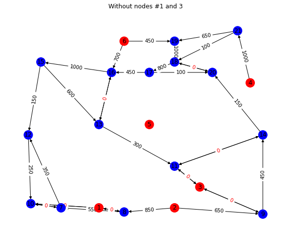
u, v = 1, 3
draw_solution(
    ampl.get_data(
        "{(i,j) in A: Build[min(i,j),max(i,j)] > 0}" + f"frns[i,j,{u},{v}]"
    ).to_dict(),
    title=f"Without nodes #{u} and {v}",
)

previous

Network Linear Programs

next

Nonlinear transportation model