Diet problem with uncertain costs

In the diet problem we want to find a diet that satisfies certain nutritional requirements while also minimizing the total cost.
What if the costs were not known exactly?
One simple approach is via robust optimization using ellipsoidal uncertainty as follows:
var t >= 0; # Auxiliary variable
minimize Total_Cost:
   sum {j in FOOD} cost[j] * Buy[j] + t; # Added to the objective
subject to Ellipsoid:
   t >= sqrt(sum {j in FOOD} (0.4 * cost[j] * Buy[j])^2); # Second-order cone
Let’s consider a simplified version of the diet problem and let’s consider uncertainty:
We have just two types of food
We just want to satisfy the required number of calories per day
The costs are not known exactly
If the costs were known exactly, we could model this problem as follows:
set NUTR;
set FOOD;

param cost {FOOD} > 0;
param calories {FOOD} >= 0;
param min_calories;
param max_calories;

var Buy {j in FOOD} >= 0;

minimize Total_Cost:
   sum {j in FOOD} cost[j] * Buy[j];

subject to Required_Calories:
   min_calories <= sum {i in FOOD} calories[i] * Buy[i] <= max_calories;
Since there is uncertainty we can do the following modifications:
var t >= 0; # Auxiliary variable
minimize Total_Cost:
   sum {j in FOOD} cost[j] * Buy[j] + t; # Added to the objective
subject to Ellipsoid:
   t >= sqrt(sum {j in FOOD} (0.4 * cost[j] * Buy[j])^2); # Second-order cone
Solving Robust and non-Robust models with MOSEK
> Not robust:
MOSEK 10.0.16: ���������������MOSEK 10.0.16: optimal; objective 8
0 simplex iterations
Buy [*] :=
BEEF 8
CHK 0
;
Total_Cost = 8
> Robust:
MOSEK 10.0.16: ���������������MOSEK 10.0.16: optimal; objective 10.4815553
0 simplex iterations
6 barrier iterations
Buy [*] :=
BEEF 4.49848
CHK 3.66268
;
Total_Cost - t = 8.16116
Solving Robust and non-Robust models with Gurobi
> Not robust:
Gurobi 10.0.1: ���������������Gurobi 10.0.1: optimal solution; objective 8
0 simplex iterations
Buy [*] :=
BEEF 8
CHK 0
;
Total_Cost = 8
> Robust:
Gurobi 10.0.1: ���������������Gurobi 10.0.1: optimal solution; objective 10.48155551
0 simplex iterations
5 barrier iterations
Buy [*] :=
BEEF 4.49905
CHK 3.66208
;
Total_Cost - t = 8.16113
We see that the robust solution balances the choices, while LP strictly prefers just 1 of the products. We exchanged some optimality for robustness.
Formal explanation
Consider a linear optimization problem of the form:
$$\min_x c^T x : Ax \ge b, \ x\ge 0$$
In practice, the objective coefficients $c$ may not be known perfectly. Assume that we only know that (with high probability) $c \in E$, where $E$ is a given ellipsoid:
$$E = { \widehat{c} + Ru : |u|_2 \le 1},$$
with center $\widehat{c} \in \mathbf{R}^n$ and $R \in \mathbf{R}^{n \times k}$. In robust optimization, we seek to minimize the objective for the worst-case scenario:
$$\max_{c \in E} c^Tx = \widehat{c}^Tx + \max_{|u|_2 \le 1} x^TR u = \widehat{c}^Tx + |R^Tx|_2,$$
where we used that $\max_{||u||_2\le1} v^Tu = (v^Tv)/||v||_2 = ||v||_2$. The robust problem is equivalent to
$$\begin{equation}
\min_x \widehat{c}^T x + ||R^Tx||_2 : Ax \ge b, \ x\ge 0.\end{equation}$$
This can be visualized for the 2D case. Assume we have two kinds of food with prices $c_1$, $c_2$ and calories per unit $a_1$, $a_2$. Buying amounts $x_1$, $x_2$ of them, we optimize the LP
\begin{align*}
\min\quad &c_1x_1 + c_2x_2
\
s.t.\quad &a_1x_1 + a_2x_2 \ge b,
\
&x_1, x_2 \ge 0.
\end{align*}
Adding an ellipsoidal uncertainty term in the objective, we obtain the problem
\begin{align*}
\min\quad &\widehat{c}_1x_1 + \widehat{c}_2x_2 + ||R^Tx||_2
\
s.t.\quad &a_1x_1 + a_2x_2 \ge b,
\
&x_1, x_2 \ge 0.
\end{align*}
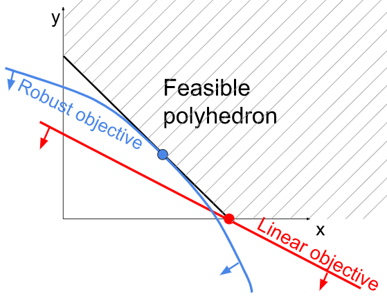
A graphical representation of the feasible set and linear vs. robust objectives:

We see that the robust solution balances the choices, while LP strictly prefers just 1 of the products.

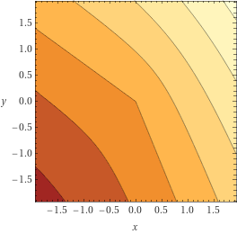
Note that the contour line passing through the origin (and corresponding to objective value 0) is piecewise-linear
The robust LP (1) can be reformulated as a conic quadratic problem:
\begin{align*}
\min \quad &\widehat{c}^T x + t
\
\text{s.t.}\quad &Ax \ge b,
\
&(t, R^Tx) \in \text{QuadCone}(n),
\ &x \ge 0.
\end{align*}