Profit Maximization for Developers: Optimizing Pricing, Marketing, and Investment Strategies#
![]()
![]()


![]()

1. Introduction#
This optimization model is designed for a real estate development project to maximize total revenue across multiple periods by managing construction, sales, advertising, and investment decisions. The project involves a portfolio of buildings under construction, each with unique characteristics such as area, start time, and construction duration.
Key components of the model include:
Construction Costs and Sales: The model tracks the progress of construction and associated monthly costs. As buildings progress, the base price per square meter of the area increases. The decision variables related to sales include the amount of area sold each month at different price steps, where price elasticity and seasonal demand impact sales potential. Advertising expenditures also influence demand, with additional square meters sold as a result of effective advertising.
Demand Elasticity: The demand for building sales is modeled using both price elasticity and seasonal effects. Price elasticity accounts for how sensitive demand is to changes in price, while seasonal effects represent demand fluctuations over time.
Revenue Calculation: Revenue is generated from the sale of square meters in each building, where the selling price depends on the selected price step and base price. The model ensures that prices either remain stable or increase over time. Additionally, advertising can boost demand, subject to a limit of increasing base demand by no more than 50%.
Advertising Expenditure: Advertising is modeled as a mechanism to increase demand, with effectiveness varying by building. The relationship between advertising and demand is nonlinear, considering the impact of seasonal demand patterns and the base price of the buildings.
Investment in Deposits: The model includes a cash management component, where the company can invest funds in deposit products of various durations (1 month, 3 months, 6 months, and 12 months). Each deposit type has its own terms, interest rates, and conditions for withdrawals and replenishments. Interest on deposits is accrued periodically, and the final balance of each deposit is calculated when it matures. The decision variables related to deposits include the amount of money invested, replenished, or withdrawn over time.
Account Balance and Cash Flow: A key constraint ensures that the company’s account balance remains non-negative throughout the planning horizon. The model tracks inflows from sales and returns from maturing deposits, while outflows include construction costs, advertising expenditures, and withdrawals from the company’s account.
Profit Maximization: The objective function seeks to maximize total revenue, calculated as the sum of account balances over all periods, taking into account sales revenue, construction costs, advertising expenses, and returns from investments in deposits.
The model also includes several key constraints to ensure feasibility, such as limiting the total area sold to the available building area, restricting the assignment of prices, and setting limits on advertising-induced demand increases. The interplay between sales decisions, advertising, and investment allows the project to maximize revenue while ensuring cash flow stability and optimizing the timing of construction and investment activities.
Tags: Marketing, Price optimization, Profitability, Residential Developer, Piecewise-linear, MIP, ampl-only, cbc
Notebook author: Mikhail Riabtsev <mail@solverytic.com>
2. Problem statement#
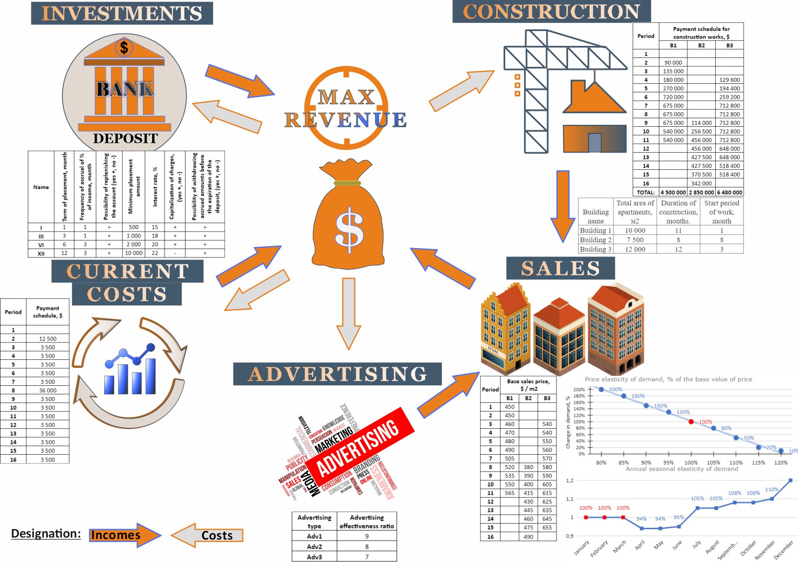
ElegantDev is embarking on an ambitious venture to create a residential complex comprising three buildings. The completion of this project is set within a 16-month timeframe as per an agreement with the city administration.
Key Indicators of buildings#
The blueprint for the residential buildings, including essential metrics, is outlined in the provided table:
| Building | |||
| B1 | |||
| B2 | |||
| B3 |
Financing Schedule#
ElegantDev has engaged various contractors for the construction and installation of the residential buildings. In accordance with the contractual obligations, the company is responsible for financing these works according to the next schedule:
| Building | ||||||||||||||||
| B1 | ||||||||||||||||
| B2 | ||||||||||||||||
| B3 | ||||||||||||||||
Nominal Sales Price#
According to current regulations, the residential units can be marketed starting one month prior to construction. Preliminary market research has established the initial sale basePrice $ per square meter, which is detailed in the accompanying table. This basePrice is subject to increase based on the construction progress.
| Building | ||||||||||||||||
| B1 | ||||||||||||||||
| B2 | ||||||||||||||||
| B3 | ||||||||||||||||
Price Elasticity of Sales#
Demand for the properties is influenced by both basePrice and seasonal factors. The Marketing Department anticipates that at the stated basePrice level (gave above), monthly nominal demand will be approximately B1:10%, B2:11%, B3:8% of the total building area.
Price changes significantly affect sales: A 20% basePrice reduction results in a doubling of sales. A 20% basePrice increase leads to a tenfold decrease in sales. Price elasticity indicators are detailed in the provided table.
| Price change, % | ||||||||
| Demand change, % |
Seasonal Elasticity of Sales#
Demand also depends on the season (time of year). Usually, the seasonal demand curve has the following form. The demand volume in the 1st month (nominal demand volume) is taken as one.
| Period, month | ||||||||||||
| Demand change, % |
Advertising Strategy#
To boost sales in the event of low demand, ElegantDev plans to leverage various advertising mediums. The efficiency of each medium is as follows:
Type A: $9 sales for every $1 spent
Type B: $8 sales for every $1 spent
Type C: $7 sales for every $1 spent
Note: The effect of advertising will be realized with a one-month delay. Advertising has a limited effect, so demand can be warmed up and increased by no more than 50%
Financial Management and Other Obligations#
ElegantDev is also handling other investment projects and has ongoing obligations. A schedule for fund withdrawals to meet these obligations is outlined in the provided schedule:
| Costs, $ | ||||||||||||||||
| Value | ||||||||||||||||
Investment Activities#
To increase the efficiency of the project, ElegantDev intends to invest available funds in financial instruments (deposits). The terms for opening new deposit accounts are detailed in the accompanying information.
Opening new deposit accounts for different types of deposits is available in the following periods:
| Deposit name | ||||||||||||||||
Objective#
Maximize developer profits by optimizing Pricing, Marketing, and Investment Strategies.#
Download Necessary Extensions and Libraries#
Let’s start by downloading the necessary extensions and libraries
# Install dependencies
%pip install -q amplpy pandas numpy
import pandas as pd  # Loading panda to work with pandas.DataFrame objects (https://pandas.pydata.org/)
import numpy as np  # Loading numpy to perform multidimensional calculations numpy.matrix (https://numpy.org/)
# Google Colab & Kaggle integration
from amplpy import AMPL, ampl_notebook

ampl = ampl_notebook(
    modules=["cbc", "highs"],  # modules to install
    license_uuid="default",  # license to use
)  # instantiate AMPL object and register magics
3. AMPL Model Formulation#
Use %%ampl_eval to evaluate AMPL commands and declarations
%%ampl_eval
reset ;
### SETS & PARAMETERS
## Construction work
param T := 16; # Planning horizon (in months)
set BUILD := {'B1','B2','B3'}; # Set of buildings under construction
set CHAR := {'area','start','duration'}; # Set of characteristics of buildings (area, start time, and construction duration)
set LINKS within {BUILD, 1..T}; # Set of building-period pairs for calculations
param buildData {BUILD, CHAR} >= 0; # Parameters for each building under construction (e.g., area, start, duration)
param buildCost {LINKS} >= 0; # Monthly construction costs for each building
param basePrice {LINKS} >= 0; # Monthly selling base Price per square meter (basePrice increases with construction progress)
param NomArea {BUILD} >= 0; # Maximum nominal sales capacity (in sq.m.) per month for each building
# Valid combinations of buildings (b) and time periods (t) where advertising demand can be considered
set LINKS_AD_DEMAND = {b in BUILD, t in buildData[b,'start']-1..(buildData[b,'start'] + buildData[b,'duration'])-1: t > 1};
## Demand (based on price and seasonal elasticity)
param nStep integer > 0; # Number of Price steps
param priceStep {1..nStep+1} >= 0; # Price step values – defining different price levels that can be set for the sale of the building area
param demandCoef {1..nStep} >= 0; # Coefficients representing price elasticity of demand for each price step. A higher coefficient means higher demand sensitivity to price changes.
param SeasonalEffect {1..T} >= 0; # Coefficient for seasonal elasticity of demand per month, representing the impact of seasonal trends on sales
# Limit on the amount of building area that can be sold in month t at price step n.
param limit {(b,t) in LINKS, n in 1..nStep} =
buildData[b,'area'] * NomArea[b] * SeasonalEffect[t] * demandCoef[n];
# The sales rate at which a certain amount of area can be sold, calculated as the product of base price and price step.
param rate {(b,t) in LINKS, n in 1..nStep} = basePrice[b,t] * priceStep[n] ;
# The incremental rate (or marginal rate) of revenue between consecutive price steps.
param marg_rate {(b,t) in LINKS, n in 1..nStep-1} =
((limit[b,t,n+1]-1) * rate[b,t,n+1] - limit[b,t,n] * rate[b,t,n]) /
(limit[b,t,n+1]-limit[b,t,n]) ;
## Advertising
param adEff {BUILD} >= 0; # Effectiveness of advertising in increasing sales per dollar invested
## Deposits
set DEP := {'I','III','VI','XII'}; # Types of deposit products (I: 1 month, III: 3 months, VI: 6 months, XII: 12 months)
# Deposit characteristics
set DEP_ATTR := {'term', 'freq_payment', 'refill', 'first_money', 'interest', 'capit_on'};
set AVAIL within {1..T, DEP}; # Availability of deposits for investment in each period
param depData {DEP, DEP_ATTR} >= 0; # Characteristics for each deposit product
# Link deposit opening periods to periods within its term
set DEP_LINKS = {(tp,d) in AVAIL, t in tp+1..tp + depData[d,'term']: t <= T+1};
# Link deposit opening periods to periods within its term (for replenishment and withdrawals)
set DEP_LINKS_ = {(tp,d,t) in DEP_LINKS: t <= T and t < tp + depData[d,'term']} ;
# Number of interest payments during the deposit term
param nInterestPayments{d in DEP} = depData[d,'term'] / depData [d, 'freq_payment'];
# Interest rate per payment period for each deposit type
param RatePerFreq{d in DEP} = (depData[d,'interest'] / 1200) * depData [d, 'freq_payment'] ;
## Cashflow & Investment schedule
param MoneyWithdrawn {1..T} >= 0 ; # Project's funds withdrawal schedule, indicating the amount of money
### DECISION VARIABLES
var SqmSold {LINKS, 1..nStep} >= 0; # Number of square meters sold for a building in a period at a given price step
var SaleDec {LINKS, 1..nStep} binary; # Binary variable indicating whether sales occurred at a given price step for a building in a period
var AdSpent {BUILD, 1..T} >= 0; # Amount of money spent on advertising for each building in each period
# AdDemand represents the additional demand generated due to advertising
# The equation multiplies the advertising spent by its effectiveness and divides it by the base price to model how much additional demand is created for each unit of advertising, adjusting for the price sensitivity of the market.
var AdDemand {(b,t) in LINKS_AD_DEMAND} =
(AdSpent[b,t-1] * # The amount of money spent on advertising for building b in the previous period (t-1)
adEff[b] / # how much demand increases per dollar spent on advertising. A higher value indicates more efficient advertising
basePrice[b,t]) * # The additional demand generated is inversely proportional to the base price. Lower base prices lead to a greater increase in demand for a given amount of advertising expenditure.
SeasonalEffect[t] ; # Coefficient for seasonal elasticity of demand per month, representing the impact of seasonal trends on sales
# Monthly profit from sales for each building in each period, considering price steps
var Monthly_Profit_From_Sales{(b,t) in LINKS} =
sum{n in 1..nStep-1} # Summation over all price steps (n) except the highest (nStep). This accumulates the total profit for each building (b) and period (t).
<< limit[b,t,n]; # Maximum amount of square meters that can be sold at price step n for building b in period t.
rate[b,t,n], # The sales rate (price per square meter) at the price step n.
marg_rate[b,t,n]>> # The marginal rate (additional profit contribution) at price step n.
SqmSold[b,t,n] + # Number of square meters sold for a building in a period at a given price step
if t > 1 then AdDemand[b,t] * basePrice[b,t]; # Sales from advertising
## Deposit variables
var IsDepositOpen {AVAIL} binary; # Binary variable indicating whether a deposit is opened
var DepositAmt {AVAIL} >= 0; # Amount invested in deposits
var ReplenishAmt {DEP_LINKS_} >= 0 ; # Amount replenished in the deposit during its term
var WithdrawalAmt{DEP_LINKS_} >= 0 ; # Amount withdrawn from the deposit during its term
# Define the accrued interest variable for each deposit product d starting in period tp.
var Accrued_Interest {(tp,d,t) in DEP_LINKS} = # % Income is calculated for each period t0. The range of t values for each t0 is within the boundaries t < t0 <= t + depData[d,'term']
# Check if the current period 't' is a scheduled interest payment period for deposit 'd'
if exists {k in 1..nInterestPayments[d]} t = tp + depData[d, 'freq_payment'] * k then
RatePerFreq[d] * DepositAmt[tp,d] + # Calculate interest for the base deposit amount
# Sum the interest from previous periods ('tt') for which interest was already accrued
# The sum includes the accrued interest over all periods 'tt' less than the current period 't'
sum{(tp,d,tt) in DEP_LINKS_: tt < t} RatePerFreq[d] *
# If the deposit 'd' has compounding (depData[d,'capit_on'] = 1), include interest accrued in previous periods
# If compounding is disabled, this part of the calculation is ignored (added as 0)
(if depData[d,'capit_on'] = 1 then Accrued_Interest[tp,d,tt] else 0 +
# If the previous period 'tt' is within one frequency payment period before 't',
# calculate the proportion of replenishment and withdrawal amounts to account for in the interest
if tt > t - depData[d, 'freq_payment'] then tt/depData[d, 'freq_payment'] *
(ReplenishAmt[tp,d,tt] # The amount replenished during period 'tt'
- WithdrawalAmt[tp,d,tt]) # The amount withdrawn during period 'tt'
# For periods 'tt' outside the current interest payment window, simply apply the full replenishment
# and withdrawal amounts without fractioning them based on the payment period frequency
else (ReplenishAmt[tp,d,tt] - WithdrawalAmt[tp,d,tt])) ;
# Define the total value of the deposit at the time of its closure (when its term ends)
# - tp: The period when the deposit was opened
# - d: The type of deposit product (e.g., 1-month, 3-month)
# - t: The period when the deposit matures (equals tp + deposit term)
# The condition `t = tp + depData[d,'term']` ensures this variable is only active when the deposit reaches its maturity.
var DepositClose {(tp,d,t) in DEP_LINKS: t = tp + depData[d,'term']} =
DepositAmt[tp,d] # Initial amount deposited when the deposit was opened
+ sum {(tp,d,tt) in DEP_LINKS} Accrued_Interest[tp,d,tt] # Add the total accrued interest over the term of the deposit.
+ sum {(tp,d,tt) in DEP_LINKS_: tt < t} # Add the total replenishment minus withdrawals over the term of the deposit, but only up to the period before the deposit closes.
(ReplenishAmt[tp,d,tt] # The amount replenished to the deposit during period tt.
- WithdrawalAmt[tp,d,tt]);
## Account Status for the Current Period
var Account {t in 1..T+1} = # The account balance at time period t, where t ranges from 1 to T+1 (including an extra period for end-of-planning balances)
sum {(b,t) in LINKS} ( # Loop over each building and time period (b,t) in the set of valid building-period pairs (LINKS)
Monthly_Profit_From_Sales[b,t] # Add the monthly profit from sales of building b in period t
- buildCost[b,t]) # Subtract the construction cost for building b in period t
- sum{b in BUILD: t <= T} AdSpent[b,t]# Subtract the advertising spent for building b in period t
- sum {(t,d) in AVAIL} DepositAmt[t,d] # Subtract the amount invested in deposits in period t for each deposit d available in that period
+ sum {(tp,d) in AVAIL: tp = t - depData[d,'term']} # Add the deposit amount from closed deposits, where tp is the opening period, and deposits close after depData[d,'term'] periods
DepositClose[tp,d,t] # Add the initial contribution of the deposit that is closing in the current period t
- sum {(tp,d,t) in DEP_LINKS_} # For each active deposit (tp, d), where tp is the opening period and t is the current period
(ReplenishAmt[tp,d,t] # Subtract the amount of money replenished into the deposit in the current period t
- WithdrawalAmt[tp,d,t]) # Subtract the amount withdrawn from the deposit in the current period t
- sum {i in 1..1: t <= T} MoneyWithdrawn[t]; # Subtract any external withdrawals (MoneyWithdrawn) in the current period t (e.g., funds withdrawn from the project for non-investment purposes)
### OBJECTIVE FUNCTION
maximize Total_revenue: sum{t in 1..T+1} Account[t] ; # Maximize total revenue by summing account balances over all periods
### CONSTRAINTS
## 1. Ensure total square footage sold does not exceed the building's area
AreaLimit_SqmSold {b in BUILD}:
sum {(b,t) in LINKS} (
(if t > 1 then AdDemand[b,t]) + sum{n in 1..nStep} SqmSold[b,t,n]) <= buildData [b,'area'];
## 2. Ensure only one price can be assigned for each period and product
PriceAssignment_Limit {(b,t) in LINKS}: sum {n in 1..nStep} SaleDec [b,t,n] <= 1;
## 3a. Constraint for monthly sales volume, considering demand, price elasticity, and seasonal effects
/*Min_MonthlySalesVolume {(b,t) in LINKS, n in 1..nStep-1}:
SqmSold[b,t,n] >= # SqmSold (square meters sold) <= Demand * Price Elasticity * Seasonal Elasticity
limit[b,t,n] * # Limit on the amount of building area that can be sold in month t at price step n
SaleDec[b,t,n] ; */ # Decision on how much to sell in period (h,t)
## 3b.
Max_MonthlySalesVolume {(b,t) in LINKS, n in 1..nStep-1}:
SqmSold[b,t,n] <=
limit[b,t,n+1] *
SaleDec[b,t,n];
## 3c. Advertising can increase demand by no more than 50% of the volume of basic demand.
# Link AdDemand & SqmSold with SaleDec
Max_MonthlySalesVolume_ {(b,t) in LINKS}:
(if t > 1 then AdDemand[b,t]) + sum{n in 1..nStep-1}(SqmSold[b,t,n]
- 1.5 * limit[b,t,n+1] * SaleDec[b,t,n]) <= 0 ;
## 4. Ensure that prices remain stable or increase throughout the sales period
stablePrice {(b,t) in LINKS: t > buildData[b,'start']-1}:
sum {n in 1..nStep} SaleDec[b,t,n] * priceStep[n] * basePrice[b,t] >= # Current period sales price.
sum {n in 1..nStep} SaleDec[b,t-1,n] * priceStep[n] * basePrice[b,t-1]; # Previous period sales price.
## 5. Ensure that the cumulative account balance is non-negative for all periods
Bal_Account_Pos {t in 1..T+1}: sum{tt in 1..t} Account[tt] >= 0;
### Deposit Constraints
## 6. Ensure the deposit amount is at least the initial required amount if a deposit is open
Min_Deposit_Amount {(t,d) in AVAIL}: DepositAmt[t,d] >= IsDepositOpen[t,d] * depData[d,'first_money'];
## 7. To limit the maximum amount that can be withdrawn from a deposit in a given period (t)
s.t. Max_Withdrawal{(tp,d,t) in DEP_LINKS_}:
WithdrawalAmt[tp,d,t] <= # The amount withdrawn at time t should not exceed:
#DepositAmt[tp,d] + # The original deposited amount is usually used as a reference, but it may be excluded here for a specific reason
sum{(tp,d,tt) in DEP_LINKS_: tt <= t} ( # The sum of accrued interest up to time t, which will be the main component determining how much can be withdrawn
Accrued_Interest[tp,d,tt] # The interest accrued on the deposit up to the current period tt
#+ ReplenishAmt[tp,d,tt] # Optionally, replenish amounts could be included, depending on whether replenishments are allowed in the withdrawal calculation
- WithdrawalAmt[tp,d,tt]) ; # Subtract previous withdrawals up to time tt to ensure the total withdrawn does not exceed the accrued interest and available balance
4. Load data from *.dat file#
%%ampl_eval
data building_developer.dat;
5. Solve problem#
Use %%ampl_eval to evaluate AMPL commands and declarations
%%ampl_eval
option solver cbc ;          # Choosing a solver
option cbc_options 'outlev=1 lim:time=30';

# Defining Output Settings
option show_stats 1 ;       # (1) Show statistical information about the size of the problem. Default 0 (statistics are not displayed)
option display_1col 0 ;     # Data Display Settings
option omit_zero_rows 1 ;   # Hide rows with 0 values. Default (0)
option omit_zero_cols 1 ;   # Hide columns with 0 values. Default (0)

solve;                      # Solve the model
Presolve eliminates 249 constraints and 249 variables.
Substitution eliminates 173 variables.
Adjusted problem:
953 variables:
	349 binary variables
	264 nonlinear variables
	340 linear variables
486 constraints; 6844 nonzeros
	17 nonlinear constraints
	469 linear constraints
	486 inequality constraints
1 nonlinear objective; 481 nonzeros.

cbc 2.10.10:
  tech:outlev = 1
  lim:time = 30
Welcome to the CBC MILP Solver
Version: 2.10.10
Build Date: Apr 18 2023

command line - Cbc_C_Interface -log 1 -solve -quit (default strategy 1)
Continuous objective value is 3.04088e+06 - 0.01 seconds
Cgl0008I 33 inequality constraints converted to equality constraints
Cgl0005I 33 SOS with 330 members
Cgl0004I processed model has 745 rows, 1348 columns (330 integer (330 of which binary)) and 5947 elements
Cbc0036I Heuristics switched off as 264 branching objects are of wrong type
Cbc0031I 174 added rows had average density of 6.2701149
Cbc0013I At root node, 174 cuts changed objective from 3040881.7 to 2359467.5 in 19 passes
Cbc0014I Cut generator 0 (Probing) - 433 row cuts average 2.6 elements, 0 column cuts (92 active)  in 0.031 seconds - new frequency is 1
Cbc0014I Cut generator 1 (Gomory) - 146 row cuts average 32.2 elements, 0 column cuts (0 active)  in 0.013 seconds - new frequency is 1
Cbc0014I Cut generator 2 (Knapsack) - 93 row cuts average 11.1 elements, 0 column cuts (0 active)  in 0.020 seconds - new frequency is 1
Cbc0014I Cut generator 3 (Clique) - 0 row cuts average 0.0 elements, 0 column cuts (0 active)  in 0.001 seconds - new frequency is -100
Cbc0014I Cut generator 4 (MixedIntegerRounding2) - 183 row cuts average 11.2 elements, 0 column cuts (0 active)  in 0.005 seconds - new frequency is 1
Cbc0014I Cut generator 5 (FlowCover) - 7 row cuts average 8.3 elements, 0 column cuts (0 active)  in 0.015 seconds - new frequency is -100
Cbc0014I Cut generator 6 (TwoMirCuts) - 503 row cuts average 70.5 elements, 0 column cuts (0 active)  in 0.030 seconds - new frequency is 1
Cbc0010I After 0 nodes, 1 on tree, -1e+50 best solution, best possible 2359467.5 (0.23 seconds)
Cbc0016I Integer solution of 2329848.7 found by strong branching after 972 iterations and 3 nodes (0.30 seconds)
Cbc0016I Integer solution of 2342977 found by strong branching after 1014 iterations and 5 nodes (0.33 seconds)
Cbc0016I Integer solution of 2346866 found by strong branching after 1134 iterations and 6 nodes (0.38 seconds)
Cbc0001I Search completed - best objective 2346865.994293246, took 1134 iterations and 6 nodes (0.38 seconds)
Cbc0032I Strong branching done 82 times (933 iterations), fathomed 3 nodes and fixed 6 variables
Cbc0035I Maximum depth 2, 306 variables fixed on reduced cost
Cuts at root node changed objective from 3.04088e+06 to 2.35947e+06
Probing was tried 35 times and created 525 cuts of which 92 were active after adding rounds of cuts (0.038 seconds)
Gomory was tried 35 times and created 157 cuts of which 0 were active after adding rounds of cuts (0.020 seconds)
Knapsack was tried 35 times and created 105 cuts of which 0 were active after adding rounds of cuts (0.032 seconds)
Clique was tried 19 times and created 0 cuts of which 0 were active after adding rounds of cuts (0.001 seconds)
MixedIntegerRounding2 was tried 35 times and created 203 cuts of which 0 were active after adding rounds of cuts (0.014 seconds)
FlowCover was tried 19 times and created 7 cuts of which 0 were active after adding rounds of cuts (0.015 seconds)
TwoMirCuts was tried 35 times and created 618 cuts of which 0 were active after adding rounds of cuts (0.040 seconds)
ZeroHalf was tried 1 times and created 0 cuts of which 0 were active after adding rounds of cuts (0.001 seconds)
ImplicationCuts was tried 16 times and created 6 cuts of which 0 were active after adding rounds of cuts (0.000 seconds)
234 bounds tightened after postprocessing


Result - Optimal solution found

Objective value:                2346865.99429325
Enumerated nodes:               6
Total iterations:               1134
Time (CPU seconds):             0.40
Time (Wallclock seconds):       0.40

Total time (CPU seconds):       0.40   (Wallclock seconds):       0.40

cbc 2.10.10: optimal solution; objective 2346865.994
1134 simplex iterations
1134 barrier iterations
6 branching nodes
assert ampl.solve_result == "solved", ampl.solve_result
6. Display the solution#
Use %%ampl_eval
%%ampl_eval
display
SqmSold, basePrice, buildCost, MoneyWithdrawn, AdSpent, Monthly_Profit_From_Sales,
Account, DepositAmt, Accrued_Interest, ReplenishAmt, WithdrawalAmt,DepositClose
;

display {(b,t) in LINKS, n in 1..nStep: SqmSold[b,t,n] > 0}
    Monthly_Profit_From_Sales[b,t] / SqmSold[b,t,n];

display {(b,t) in LINKS, n in 1..nStep-1: SaleDec[b,t,n] > 0}(
    limit[b,t,n],
    limit[b,t,n+1],
    SqmSold[b,t,n]
    );
SqmSold [B1,*,*]
:     3     :=
1    500
2    500
3    500
4    752
5    752
6    760
7    840
8    840
9    864
10   864
11   880

 [B2,*,*]
:      4      :=
8    693
9    712.8
10   712.8
11   726
12   792
13   660
14   660
15   660
16   620.4

 [B3,*,*]
:      4       :=
3    768
4    721.92
5    721.92
6    729.6
7    806.4
8    806.4
9    829.44
10   829.44
11   844.8
12   921.6
13   768
14   768
15   768
;

:     basePrice buildCost    :=
B1 1      450          0
B1 2      450      90000
B1 3      460     135000
B1 4      470     180000
B1 5      480     270000
B1 6      490     720000
B1 7      505     675000
B1 8      520     675000
B1 9      535     675000
B1 10     550     540000
B1 11     565     540000
B2 8      380          0
B2 9      390     114000
B2 10     400     256500
B2 11     415     456000
B2 12     430     456000
B2 13     445     427500
B2 14     460     427500
B2 15     475     370500
B2 16     490     342000
B3 3      540          0
B3 4      540     129600
B3 5      550     194400
B3 6      560     259200
B3 7      570     712800
B3 8      580     712800
B3 9      590     712800
B3 10     605     712800
B3 11     615     712800
B3 12     625     648000
B3 13     635     648000
B3 14     645     518400
B3 15     655     518400
;

MoneyWithdrawn [*] :=
 2 12500    5  3500    8 36000   11  3500   14  3500
 3  3500    6  3500    9  3500   12  3500   15  3500
 4  3500    7  3500   10  3500   13  3500   16  3500
;

:       AdSpent  Monthly_Profit_From_Sales    :=
B1 1        0               247500
B1 2        0               247500
B1 3        0               253000
B1 4        0               370618
B1 5        0               378504
B1 6    11970.4             390506
B1 7    23111.1             558000
B1 8    23777.8             676494
B1 9    24444.4             715910
B1 10   25111.1             735982
B1 11       0               770067
B2 8        0               276507
B2 9        0               291892
B2 10       0               299376
B2 11       0               316354
B2 12       0               357588
B2 13   33206.3             308385
B2 14   34289.1             584430
B2 15    7037.23            603488
B2 16       0               372116
B3 3        0               435456
B3 4        0               409329
B3 5        0               416909
B3 6        0               429005
B3 7        0               482630
B3 8        0               491098
B3 9        0               513838
B3 10       0               526902
B3 11   60000               545530
B3 12       0              1108800
B3 13   21937.4             512064
B3 14   62880               673690
B3 15       0               968352
;

Account [*] :=
 1      -2.91038e-11    8      -4.88944e-09   14  211551
 2      -2.91038e-11    9      -7.45058e-09   15 -211551
 4      -2.91038e-09   10      -3.72529e-09   16       1.39698e-09
 5       4.13274e-09   11      -6.51926e-09   17 2346870
 6      -2.56114e-09   12       6.98492e-10
 7      -1.39698e-09   13      -9.31323e-10
;

DepositAmt [*,*]
:        I           III         VI      :=
1         0        247500        .
2         0        145000        .
3         0        549956        .
4         0        368138      348684
5         0             0      473963
6         0          3956.66   376339
8       167.536         0           0
10    68626.4      310589           0
11   409028             0           0
12        0       1150260           0
;

:         Accrued_Interest ReplenishAmt WithdrawalAmt  DepositClose    :=
1  III 4      2475                .            .         249975
2  III 5      1450                .            .         146450
3  III 6      5499.56             .            .         555456
4  III 7      3681.38             .            .         371820
4  VI  7      3922.69               0      1961.35           .
4  VI  8         0                  0       980.673          .
4  VI  9         0                  0       490.337          .
4  VI  10     3966.82             .            .         353141
4  XII 15        0            2045710         0              .
4  XII 16   127857                .            .        2173570
5  VI  8      5332.08               0      2666.04           .
5  VI  9         0                  0      1333.02           .
5  VI  10        0                  0       666.51           .
5  VI  11     5392.07             .            .         480021
5  XII 16        0            2200190         0              .
5  XII 17   146679                .            .        2346870
6  III 9        39.5666           .            .           3996.23
6  VI  9      4233.81               0      2116.91           .
6  VI  10        0                  0      1058.45           .
6  VI  11        0                  0       529.226          .
6  VI  12     4281.44             .            .         381149
8  I   9         0.488648         .            .            168.025
10 I   11      200.16             .            .          68826.6
10 III 13     3105.89             .            .         313695
11 I   12     1193                .            .         410221
12 III 15    11502.6              .            .        1161760
;

Monthly_Profit_From_Sales[b,t]/SqmSold[b,t,n] [*,*,3] (tr)
:      B1       :=
1    495
2    495
3    506
4    492.844
5    503.33
6    513.823
7    664.285
8    805.35
9    828.6
10   851.832
11   875.076

 [*,*,4] (tr)
:      B2        B3       :=
3       .       567
4       .       567
5       .       577.5
6       .       588
7       .       598.5
8    399        609
9    409.5      619.5
10   420        635.25
11   435.75     645.75
12   451.5     1203.12
13   467.25     666.75
14   885.5      877.2
15   914.375   1260.88
16   599.8         .
;

:       limit[b,t,n] limit[b,t,n + 1] SqmSold[b,t,n]    :=
B1 1  3     500            800             500
B1 2  3     500            800             500
B1 3  3     500            800             500
B1 4  3     470            752             752
B1 5  3     470            752             752
B1 6  3     475            760             760
B1 7  3     525            840             840
B1 8  3     525            840             840
B1 9  3     540            864             864
B1 10 3     540            864             864
B1 11 3     550            880             880
B2 8  4     693            866.25          693
B2 9  4     712.8          891             712.8
B2 10 4     712.8          891             712.8
B2 11 4     726            907.5           726
B2 12 4     792            990             792
B2 13 4     660            825             660
B2 14 4     660            825             660
B2 15 4     660            825             660
B2 16 4     620.4          775.5           620.4
B3 3  4     768            960             768
B3 4  4     721.92         902.4           721.92
B3 5  4     721.92         902.4           721.92
B3 6  4     729.6          912             729.6
B3 7  4     806.4         1008             806.4
B3 8  4     806.4         1008             806.4
B3 9  4     829.44        1036.8           829.44
B3 10 4     829.44        1036.8           829.44
B3 11 4     844.8         1056             844.8
B3 12 4     921.6         1152             921.6
B3 13 4     768            960             768
B3 14 4     768            960             768
B3 15 4     768            960             768
;
7. Retrieve solution in Python and save data in *.json#
import json

# Initialize an empty dictionary to store AMPL variable data
amplvar = dict()

# Prepare a list of AMPL variables (assuming ampl.get_variables() is a function that retrieves variable data)
list_of_ampl_variables = [item[0] for item in ampl.get_variables()]

# Iterate over each variable name in the list
for key_ampl in list_of_ampl_variables:
    # Skip certain variables that are not to be processed (these variables won't be included in the output)
    if key_ampl not in [""]:
        # Convert the AMPL variable data to a pandas DataFrame
        df = ampl.var[key_ampl].to_pandas()
        # Filter the DataFrame to include only rows where the variable's value is greater than a small threshold (1e-5)
        filtered_df = df[df[f"{key_ampl}.val"] > 1e-5]
        # Round the values in the DataFrame to two decimal places
        rounded_df = filtered_df.round(2)
        # Convert the filtered DataFrame to a dictionary and add it to the amplvar dictionary
        amplvar[key_ampl] = filtered_df.to_dict(orient="records")
        display(rounded_df)
# Save the entire dictionary to a JSON file
with open("dataframes.json", "w") as file:
    json.dump(amplvar, file, indent=4)
| Account.val | |
|---|---|
| 14 | 211550.54 |
| 17 | 2346865.99 |
| Accrued_Interest.val | |||
|---|---|---|---|
| index0 | index1 | index2 | |
| 1 | III | 4 | 2475.00 |
| 2 | III | 5 | 1450.00 |
| 3 | III | 6 | 5499.56 |
| 4 | III | 7 | 3681.38 |
| VI | 7 | 3922.69 | |
| 10 | 3966.82 | ||
| XII | 16 | 127857.12 | |
| 5 | VI | 8 | 5332.08 |
| 11 | 5392.07 | ||
| XII | 17 | 146679.12 | |
| 6 | III | 9 | 39.57 |
| VI | 9 | 4233.81 | |
| 12 | 4281.44 | ||
| 8 | I | 9 | 0.49 |
| 10 | I | 11 | 200.16 |
| III | 13 | 3105.89 | |
| 11 | I | 12 | 1193.00 |
| 12 | III | 15 | 11502.59 |
| AdDemand.val | ||
|---|---|---|
| index0 | index1 | |
| B1 | 7 | 224.00 |
| 8 | 420.00 | |
| 9 | 432.00 | |
| 10 | 432.00 | |
| 11 | 440.00 | |
| B2 | 14 | 577.50 |
| 15 | 577.50 | |
| 16 | 108.00 | |
| B3 | 12 | 806.40 |
| 14 | 238.08 | |
| 15 | 672.00 |
| AdSpent.val | ||
|---|---|---|
| index0 | index1 | |
| B1 | 6 | 11970.37 |
| 7 | 23111.11 | |
| 8 | 23777.78 | |
| 9 | 24444.44 | |
| 10 | 25111.11 | |
| B2 | 13 | 33206.25 |
| 14 | 34289.06 | |
| 15 | 7037.23 | |
| B3 | 11 | 60000.00 |
| 13 | 21937.37 | |
| 14 | 62880.00 |
| DepositAmt.val | ||
|---|---|---|
| index0 | index1 | |
| 1 | III | 247500.00 |
| 2 | III | 145000.00 |
| 3 | III | 549956.00 |
| 4 | III | 368138.23 |
| VI | 348683.91 | |
| 5 | VI | 473962.80 |
| 6 | III | 3956.66 |
| VI | 376338.83 | |
| 8 | I | 167.54 |
| 10 | I | 68626.45 |
| III | 310588.73 | |
| 11 | I | 409028.06 |
| 12 | III | 1150258.56 |
| DepositClose.val | |||
|---|---|---|---|
| index0 | index1 | index2 | |
| 1 | III | 4 | 249975.00 |
| 2 | III | 5 | 146450.00 |
| 3 | III | 6 | 555455.56 |
| 4 | III | 7 | 371819.61 |
| VI | 10 | 353141.07 | |
| XII | 16 | 2173571.07 | |
| 5 | VI | 11 | 480021.38 |
| XII | 17 | 2346865.99 | |
| 6 | III | 9 | 3996.23 |
| VI | 12 | 381149.50 | |
| 8 | I | 9 | 168.03 |
| 10 | I | 11 | 68826.61 |
| III | 13 | 313694.62 | |
| 11 | I | 12 | 410221.06 |
| 12 | III | 15 | 1161761.14 |
| IsDepositOpen.val | ||
|---|---|---|
| index0 | index1 |
| Monthly_Profit_From_Sales.val | ||
|---|---|---|
| index0 | index1 | |
| B1 | 1 | 247500.00 |
| 2 | 247500.00 | |
| 3 | 253000.00 | |
| 4 | 370618.50 | |
| 5 | 378504.00 | |
| 6 | 390505.50 | |
| 7 | 557999.75 | |
| 8 | 676494.00 | |
| 9 | 715910.25 | |
| 10 | 735982.50 | |
| 11 | 770066.75 | |
| B2 | 8 | 276507.00 |
| 9 | 291891.60 | |
| 10 | 299376.00 | |
| 11 | 316354.50 | |
| 12 | 357588.00 | |
| 13 | 308385.00 | |
| 14 | 584430.00 | |
| 15 | 603487.50 | |
| 16 | 372115.80 | |
| B3 | 3 | 435456.00 |
| 4 | 409328.64 | |
| 5 | 416908.80 | |
| 6 | 429004.80 | |
| 7 | 482630.40 | |
| 8 | 491097.60 | |
| 9 | 513838.08 | |
| 10 | 526901.76 | |
| 11 | 545529.60 | |
| 12 | 1108800.00 | |
| 13 | 512064.00 | |
| 14 | 673689.60 | |
| 15 | 968352.00 |
| ReplenishAmt.val | |||
|---|---|---|---|
| index0 | index1 | index2 | |
| 4 | XII | 15 | 2045713.95 |
| 5 | XII | 16 | 2200186.87 |
| SaleDec.val | |||
|---|---|---|---|
| index0 | index1 | index2 | |
| B1 | 1 | 3 | 1.0 |
| 2 | 3 | 1.0 | |
| 3 | 3 | 1.0 | |
| 4 | 3 | 1.0 | |
| 5 | 3 | 1.0 | |
| 6 | 3 | 1.0 | |
| 7 | 3 | 1.0 | |
| 8 | 3 | 1.0 | |
| 9 | 3 | 1.0 | |
| 10 | 3 | 1.0 | |
| 11 | 3 | 1.0 | |
| B2 | 8 | 4 | 1.0 |
| 9 | 4 | 1.0 | |
| 10 | 4 | 1.0 | |
| 11 | 4 | 1.0 | |
| 12 | 4 | 1.0 | |
| 13 | 4 | 1.0 | |
| 14 | 4 | 1.0 | |
| 15 | 4 | 1.0 | |
| 16 | 4 | 1.0 | |
| B3 | 3 | 4 | 1.0 |
| 4 | 4 | 1.0 | |
| 5 | 4 | 1.0 | |
| 6 | 4 | 1.0 | |
| 7 | 4 | 1.0 | |
| 8 | 4 | 1.0 | |
| 9 | 4 | 1.0 | |
| 10 | 4 | 1.0 | |
| 11 | 4 | 1.0 | |
| 12 | 4 | 1.0 | |
| 13 | 4 | 1.0 | |
| 14 | 4 | 1.0 | |
| 15 | 4 | 1.0 |
| SqmSold.val | |||
|---|---|---|---|
| index0 | index1 | index2 | |
| B1 | 1 | 3 | 500.00 |
| 2 | 3 | 500.00 | |
| 3 | 3 | 500.00 | |
| 4 | 3 | 752.00 | |
| 5 | 3 | 752.00 | |
| 6 | 3 | 760.00 | |
| 7 | 3 | 840.00 | |
| 8 | 3 | 840.00 | |
| 9 | 3 | 864.00 | |
| 10 | 3 | 864.00 | |
| 11 | 3 | 880.00 | |
| B2 | 8 | 4 | 693.00 |
| 9 | 4 | 712.80 | |
| 10 | 4 | 712.80 | |
| 11 | 4 | 726.00 | |
| 12 | 4 | 792.00 | |
| 13 | 4 | 660.00 | |
| 14 | 4 | 660.00 | |
| 15 | 4 | 660.00 | |
| 16 | 4 | 620.40 | |
| B3 | 3 | 4 | 768.00 |
| 4 | 4 | 721.92 | |
| 5 | 4 | 721.92 | |
| 6 | 4 | 729.60 | |
| 7 | 4 | 806.40 | |
| 8 | 4 | 806.40 | |
| 9 | 4 | 829.44 | |
| 10 | 4 | 829.44 | |
| 11 | 4 | 844.80 | |
| 12 | 4 | 921.60 | |
| 13 | 4 | 768.00 | |
| 14 | 4 | 768.00 | |
| 15 | 4 | 768.00 |
| WithdrawalAmt.val | |||
|---|---|---|---|
| index0 | index1 | index2 | |
| 4 | VI | 7 | 1961.35 |
| 8 | 980.67 | ||
| 9 | 490.34 | ||
| 5 | VI | 8 | 2666.04 |
| 9 | 1333.02 | ||
| 10 | 666.51 | ||
| 6 | VI | 9 | 2116.91 |
| 10 | 1058.45 | ||
| 11 | 529.23 |
8. Enhancements#
Try to explain why the model chooses in most cases the extreme values of demand (min or max) for the chosen price?
What are the reasons for the model choosing intermediate values of demand for the chosen price?